Component 145: Stratified Storage

In This Topic

Component 145: Stratified Storage

Specifications

Line connections (ports)
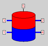
1	Fluid inlet when discharging the storage tank
2	Fluid outlet when discharging the storage tank
3	Fluid inlet when charging the storage tank
4	Fluid outlet when charging the storage tank
5	Logic Outlet: heat transfer between fluid and storage as enthalpy h

Before Release 16 (obsolete) there were only three ports:

1 (medium inlet), 2 (medium outlet) and 3 (logic connection for the amount of heat exchanged during the time step) available. Port 1 was meant for unloading in the lower ("cold") part of the tank and for loading in the upper ("warm") part of the tank. Port 2 was meant for unloading in the upper ("warm") part of the storage tank and for loading in the lower ("cold") part of the storage tank. To calculate with the old logic, you can either work with FCHARGE=0 or FCHARGE=1. Existing models do not need to be adapted.

General User Input Values Physics Used Displays Example

General

The component “Stratified storage” describes a tank filled with a fluid which, depending on the initial/boundary conditions, can have a thermo cline. Mass and energy balances are calculated in such a way that they represent a storage system for thermal energy. The special feature of this component is its transient functionality . EBSILON^®Professional simulates the charging and discharging function whereby, in contrast to Component 118, no ideal mixture of the content of the storage tank (like e.g. in a stirrer tank) is simulated. In doing so, the thermal stratification is preserved space-resolved and varies with the charging condition over the storage height. Thermal losses to the environment can be accounted for. In analogy to Component 119, these are dynamically included in the calculation as a function of the occurring temperature gradients. In combination with the time series calculation dialog, transient calculations of the thermal storage system can be modelled.

The condition of the storage tank (temperature, position of the thermo cline) is accessible via specification and result values. To be able to access corresponding variables also during the calculation (e.g. for a closed-loop control), a logic outlet has been added.

On Outlet 5, the heat flow charged and discharged respectively over the time step is output:

Charged/discharged heat flow as enthalpy h

Please note: A change of these variables over the course of the calculation has nothing to do with the chronological sequence, but with the behaviour of the iteration.

Implementation and Monitoring of the Dimensionless Diffusion Number

In this Component, the precision and the stability of the numerical solution depend on the number NFLOW of grid points in the height as well as on the width of the time steps (e.g. in the time series). For this, a dimensionless number, the diffusion criterion RDIFNUMB, has been implemented. For a robust numerical solution, the respective parameters, NFLOW and time step, have to be selected by the user in such a way that the result value RDIFNUMB remains < 0.8. If the value of RDIFNUMB exceeds the limit of 0.8, the user will be warned with an error message.

User Input Values

FINIT	Initializing state =0: Global (calculation control over TRANSIENTMODE) =1: First run =2: Continuation run
FLAM	Specification of thermal conductivity (fluid in storage) =0: Calculation from property tables =1: By specification value LAMFLUID (constant) =2: Lambda fluid neglected
LAMFLUID	Thermal conductivity fluid in storage
CORRCONV	Correction term for heat conduction in storage fluid
FCHARGE	Specification of load/unload control =0: (obsolete, for old model when there were only three ports) Externally by value LFLAG =1: (obsolete, for old model when there were only three ports) Using gradient of temperature =2: via LFLAG, unloading via flow path 1->2, loading via flow path 3->4
FDP	Pressure handling = 1: Use geometry =-1: P1 and P2 given from outside
FVOL	Definition of storage geometry =0: By volume and height =1: By height and cross section =2: By volume and cross section
HEIGHT	Height of storage
ASECT	Cross section of storage
VCAP	Volume at full state
THSTO	Wall Thickness
RHO	Density of the storage walls
LAM	Thermal conductivity of the storage walls
CP	Specific heat of the storage walls
THISO	Thickness of insulation
LAMISO	Thermal conductivity of insulation
ALPHI	Inner heat transfer coefficient (to fluid)
ALPHO	Outer heat transfer coefficient (to ambient)
NFLOW	Number of grid points in height (flow direction)
FSTART	Specification of start temperature =1: Set only wall temperature from TSTART =2: From stationary solution =3: Set wall and fluid temperature from TSTART =4: Function for thermo cline with geometric positions =5: Function for thermo cline percentage
TSTART	Start temperature
POSTEMP1	First (lower) position of initial thermo cline - POSTEMP2 > POSTEMP1
POSTEMP2	Second (upper) position of initial thermo cline
TTOL	Temperature tolerance for triggering load changes
PLOAD	Superimposed pressure
FSTAMB	Definition of ambient temperature =0: Specification value TAMB =1: Defined from superior model
TAMB	Ambient temperature
ISUN	Index for solar parameters
LFLAG	Flag loading storage

Generally, all inputs that are visible are required. But, often default values are provided.

For more information on colour of the input fields and their descriptions see Edit Component\Specification values

For more information on design vs. off-design and nominal values see General\Accept Nominal values

Result values

TAVBEG	Average temperature of storage in the beginning of time step
TAVEND	Average temperature of storage in the end of time step
T2BEG	Outlet temperature of fluid in the beginning of time step
T2END	Outlet temperature of fluid in the end of time step
RTAMB	Ambient temperature used in calculation
QSTO	Energy stored during time step
QAV	Average energy flow in time step
QAVO	Average energy flow from storage to environment
HFLAV	Average enthalpy in fluid
TFLAV	Average temperature in fluid
PFLAV	Average pressure in fluid
RVFLUID	Used flow volume of fluid
DPGEOD	Pressure loss from geodesic height
RHEIGHT	Calculated from geometry
RPOSTC	Calculated position of thermo cline
RTAUSTO	Calculated time constant of fluid in storage
RLFLAG	Status of Storage charging: (0=discharging, 1=charging): RLFLAG=0: Storage is being discharged RLFLAG=1: Storage is being loaded
RDIFNUMB	Dimensionless diffusion number ( FINIT>1 only)

Specification matrix MXTSTO and result matrix RXTSTO

The matrix MXTSTO is linked to the output field RXTSTO in the same way as the characteristic curves and result curves mentioned above.

The distribution of the values in the storage and the fluids is stored in both matrices (default matrix MXTSTO for time step t-1 and result matrix RXTSTO for time step t).

For the structure of the matrices, see matrices of component 145.

Physics used

Equations

Definition of the initial conditions, temperature profile of the storage tank

The user has the following options for defining the initial temperature profile of the fluid in the storage tank and the storage wall. The flag FSTART offers various options for the initialization:

FSTART=1: Only the storage wall is set to TSTART, the fluid temperature is taken over from the specification at Pin 1.
FSTART=2: The steady-state solution is calculated for calculating the temperatures.
FSTART=3: Storage wall and fluid are set to the temperature TSTART
FSTART=4: Specification of a thermo cline

Flag position 4 assumes that the temperature profile in the storage tank can be described with a hyperbolic tangent function. The following illustration shows in an exemplary way a typical behaviour of the temperature over the storage height:

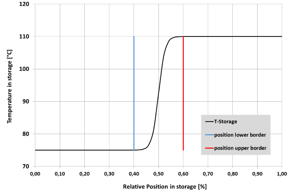
Figure 1: Thermo Cline

Four parameters are included in the calculation. Two geometrical positions (POSTEMP1 - lower, POSTEMP2 - upper), which define the position and thickness of the thermo cline, and the two temperatures TSTART and the temperature of the fluid entering the storage tank, between which the temperature profile forms. As the illustration shows, the change of the storage temperature begins at the position POSTEMP1 and ends at POSTEMP2, whereby the inflection point of the hyperbolic tangent function is always located in the middle between these two points. At this position there is the arithmetic mean of the two specified temperatures.

To the greatest extent, the transient calculation is effected with the algorithms of Component 119. The combined model containing numerical and analytic approaches is used. The consideration of the fluid mass as component of the storage is fixed, just as the possibility to receive different mass flows at inlet and outlet. In addition, the axial heat conduction in the fluid is included in the calculation; depending on the user’s requirements, it can be “augmented” with a convective portion via the specification value CORRCONV.

Control of the calculation sequence

As a rule, the transient simulation in this component is controlled via the EBSILON^®Professional time series dialog. Here the flag FINIT serves to control the calculation modes.

“Global“ : The component is controlled via the model variable “Transient” (in the dialog ”Extras“->”Model Options”->”Simulation“->combo box "Transient").
„First Run" : executes the initialization according to the user’s specification (see flag FSTART).
„Continuation Run“ effects the actual transient simulation, whereby the results of the previous time step are passed on as input parameters for the following step in each case.

Besides using the time series dialog, individual simulations can be initiated as well (button ”Simulate“ or F9). Here the component is influenced by the model variable “Time handling“ as follows:

„steady state“ : Only a steady-state calculation is carried out (in the dialog ”Extras“->”Model Options“->”Simulation“->combo box ”Time handling“)
„calculate maximum“ and „set maximum / upper bound“ do not have the same effects here as in Component 118! A single transient simulation with the specified time interval is carried out.
„Continuation Run“ effects the actual transient simulation, whereby the results of the previous time step are passed on as input parameters of the following step in each case.

Mass balance

During the integration time interval, the incoming and outgoing mass flows at Port “1” are constant but not necessarily equal. According to possible changes in the density of the fluid, the new mass in the storage tank is calculated and can be retrieved via the two corresponding diagrams CMFL and RAMFL as well as the result variable MFLUID. This happens simultaneously with the solving of the energy balance.

Energy balance

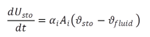
The energy balance of the storage system can be formulated globally as follows:

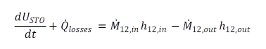(1)

The chronological change of the internal energy of the storage tank plus lost heat flow to the environment corresponds to the change of the enthalpy of the inflowing and out flowing fluid. In the calculation of U_sto it is invariably specified that the fluid and its thermal mass respectively has a share in the stored energy. Thus it is possible to formulate for the fluid and the storage tank:

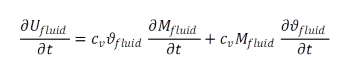	(2)
	(3)

For a simplification for solving this equation for the storage tank, the following assumption is made. A discretisation of the component is effected according to user specification via the component height. Radially, the wall and the fluid itself are only represented with one element in each case. In analogy to Component 119 the local resolution of the computational grid is effected radially symmetrically in 2D. The following illustration shows the schematic structure of the model:

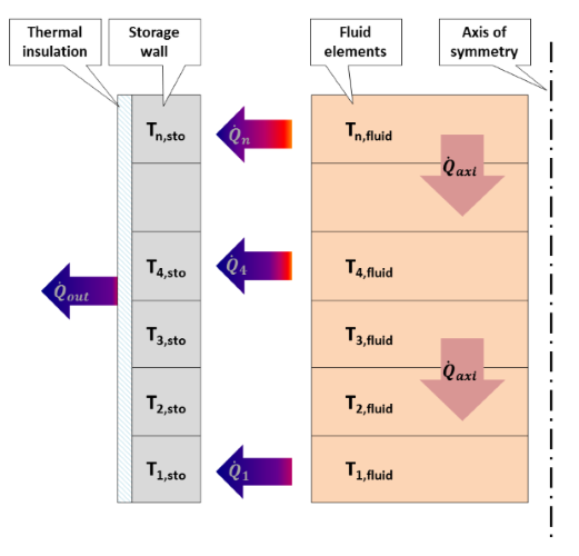
Figure 2: Schematic structure of the calculation model

This pattern is also found in the representation of the calculated temperatures in the matrix RXTSTO. Like in the other transient, space-resolved components, the insulation of the storage tank is not discretized and thus only represents an additional thermal resistance which itself, however, does not possess any storage-capable mass. Here the individual fluid elements are also thermally in contact with each other to allow to consider the occurrence of axial heat conduction. The adjacent wall elements, however, are not connected as that would require the much more complex Crank-Nicolson algorithm. Without this interconnection, an analytic approach can be made for the dynamic simulation:

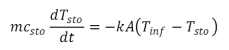	(4)
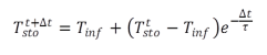	(5)

As no temperature gradients occur within a discretisation element, this approach can be integrated directly and we receive the form of the solution for the storage temperature as a function of the time step width shown in Equation (5). The two temperatures with the index “sto“ describe the condition of the storage tank before and after the time interval Dt, here T_inf as a driving force describes the steady-state final temperature of the storage tank, and t is the storage time constant mc/kA. The energy balance coupled with the fluid is solved numerically, iteratively by means of Equation (2).

Momentum balance

Depending on the specification by the user, the pressure in the storage tank is set by the flag position FDP and calculated according to the geometrical conditions respectively.

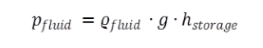„Use geometry“ : Via storage height and fluid density, calculated according to the formula for the geodetic pressure:

(6)

Please note: The density of the fluid changes with its temperature and thus on the one hand depends on the stratification, on the other hand also chronological changes are possible depending on the mode of operation of the storage tank. While during “discharging” the entire pressure of the water column in the tank weighs on the inflowing cold fluid, the hot fluid flowing out of the storage tank is subject to a changed pressure change. The density at out flowing conditions in Equation (4) is taken over. During “charging“ there are analogous conditions, i.e. the water column always weighs on the cold fluid to its full extent.
„P1 and P2 given from outside“ : Both pressures can be set by the user freely and independently of each other.

In addition to the given pressures, an additional pressurization can be effected for certain storage types by means of the specification value PLOAD. It is treated by the model as absolute pressure.

Please note: If the thermodynamic conditions lead to a phase change in the storage tank, an error message will be output!

Storage model and time series calculation dialog

Besides the conventional “calculation“ feature, for Component 145 EBSILON^®Professional also offers the option to simulate a time series. Within the time series dialog, the user can either specify fixed values (temperature, mass flow) for the inlet line or simulate the behaviour of the stratified storage tank in conjunction with other components.

Depending on the choice how the charging status is checked, the flag LFLAG for charging/discharging will have to be set additionally. If the temperature of the fluid flowing into the storage tank is below the mean value occurring in the thermo cline (plus a specifiable tolerance TTOL), the discharging process will be simulated. This means that the storage tank is configured in such a way that fluid is removed from the hot head section via Pin “2“. This feature is also available as an automatism. It is guided by the conditions that existed on the inlet line at the end of the previous time step. If a change of the fluid temperature across the tolerance limit occurs, the calculation mode will be switched over to the respective opposite state.

Please note: Here it is important to mind the consistency of the boundary conditions when manually defining the storage condition! When the storage tank is discharged, the control variable LFLAG must be set to “0“ and, in the opposite case, when charging with hot fluid to “1“, otherwise physically unreasonable stratifications and violations of the energy balance may occur!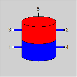

Component Displays

Display Option 1

Example

Click here >> Component 145 Demo << to load an example.