
EBSILON®Professional Online Documentation


|
Line Connections |
|
|
|
1 |
Fluid inlet |
|
|
2 |
Fluid outlet |
|
|
3 |
Heat extraction from fluid to storage medium |
|
General User Input Values Physics Used Characteristic Lines Results Displays Example
This component provides fast access to the representation of non-steady state processes in Ebsilon. Although by principle, Ebsilon is limited to steady-state solutions because the component equations do not contain a time-dependency and Ebsilon thus solves a steady state equation system, this component allows the representation of non-steady state processes like e.g.
by adding respective sources and sinks:
 |
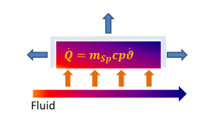
The component "indirect storage" calculates the non-steady state heat exchange of the material with the fluid that flows through and around it, respectively. For this, the structure flown through is represented by a pipe model of similar mass, heat exchanger surface, and material characteristics. The influence of the kind of flow and the geometry of the actual structure on the heat transfer is taken into consideration by the heat transfer coefficient α at the heat transfer surface inside the pipe. The modeling as a pipe has the advantage that a large number of technical applications can be translated to the theory of the heat transfer in pipes. Another advantage of the pipe geometry consists in the cycle-symmetric temperature distribution and heat transfer, so that the calculation of the temperature field is reduced to a cross-section along the direction of flow.
Based on an initial state of the temperature field, component 119 calculates the change of the temperature field of the pipe due to a change of the determining factors within a defined period of time. The determining factors are defined by the specification values of the component as well as by the state variables of the fluid at the component inlet. The component has to be used in combination with the time series calculation in which the calculation period is defined and by means of which the determining factors for defined points in time can be changed. During a calculation step in the time series calculation, the specification values and state variables of the model remain constant.
The FDP switch was introduced for this purpose. With
The geometry-based pressure loss calculation only makes sense if the component 119 models a real pipe. In this case, the inner diameter DIAI, the pipe length LSTO and the wall roughness KS are used to calculate the pressure loss in addition to the volume flow of the medium.
|
FMODE |
Flag: Calculation mode (design / off-design) =0: Global |
|
FINIT
|
Flag: Initializing state =0: Global, which is controlled via global variable "Transient mode" under Model Options =1: First run -> Initializing while calculating steady state values |
|
FINST
|
Flag: Determination of transient calculation modes = 0: Transient solution according to time series table |
|
FALGINST
|
Flag: Determination of transient calculation algorithms |
| FGTYP |
Typ der Speicherwandgeometrie-Vorgabe =0: Rohr |
|
FSTO |
Flag: Definition of storage geometry =0: By LSTO, ASTO and MSTO |
|
LSTO |
Flow length of storage |
|
DIAI |
Inner diameter of storage pipe |
|
THSTO |
Thickness of storage pipe |
|
ASTO |
Heat exchanging area of storage |
|
MSTO |
Mass of storage |
|
FVFLUID |
Determination of the fluid volume that defines the fluid mass at a given fluid density =0: Fluid volume defined by VFLUID |
|
VFLUID |
Flag: Switch for calculation of fluid volumes =0: Given from specification VFLUID |
| FMAT |
Wall material see Steel Grades |
|
FDATA |
Flag: Data source and interpolation = 1: Constant from specification values RHO, LAM, CP |
|
RHO |
Density of storage at TREF, or constant and independent of TREF in case of FDATA = 1 |
|
DRHO |
Density change per degree defines the gradient of the linear function FDATA=2 |
|
LAM |
Heat conductivity of storage at TREF, or constant and independent of TREF in case of FDATA = 1 |
|
DLAM |
Heat conductivity change per degree defines the gradient of the linear function FDATA=2 |
|
CP |
Spezific heat capacity of storage at TREF, or constant and independent of TREF in case of FDATA = 1 |
|
DCP |
Change of specific heat capacity per degree defines the gradient of the linear function FDATA=2 |
| ERHO | Function for material density |
| ELAM | Function for material heat conductivity |
| ECP | Function for material heat capacity |
|
TREF |
Reference temperature for RHO, LAM, CP when FDATA=2 |
|
THISO |
Thickness of insulation |
|
LAMISO |
Heat conductivity of insulation |
|
TAUADJ |
Correction factor for the time constant of the wall (reduced physical model only) |
|
LAMADJ |
Multiplication factor to 1/LAMBDA - the walls heat conductivity resistance (reduced physical model only) Setting LAMADJ=0 is equivalent to neglecting the walls heat conductivity resistance: either the wall thickness is infinitely small or lambda value is infinitely high Setting LAMADJ=1 is equivalent to computing the walls heat conductivity with the original value of LAMBDA and wall thickness LAMADJ<1 leads to decreasing the walls heat conductivity resistance LAMADJ>1 leads to increasing the walls heat conductivity resistance |
|
FSPECM |
Flag: Handling of fluid mass = 1: Fluid mass neglectible |
|
FTTI |
Flag: Handling of temperature during time interval =0: Actual temperature at the end of time step |
|
FTSTEPS |
Flag: Specification of (sub-) time steps =1: By specification value TISPEP |
|
ISUBMAX |
Maximum number of time sub steps for initialization |
|
IERRMAX |
Maximum allowed error for initializing step |
|
TISTEP |
Time step |
| FNUMSC |
Numeric scheme =0: Upwind |
|
NFLOW |
Number of points in x-direction (max. 100) in flow direction. When FSPECM=4 NX is fixed to =1 |
|
NRAD |
Number of points in y-direction (max. 30) in radial direction |
|
TIMESING |
Integration time for single calculation when FINST=2 |
|
FFREQ
|
Flag: Frequency of transient calculation =1: At each iteration step |
|
FSTART
|
Flag: Specification of start temperature =1: From specification value TSTART |
|
TSTART |
Start temperature when FSTART=1 |
|
TMIN |
Lower limit for storage temperature |
|
TMAX |
Upper limit for storage temperature |
|
FSTAMB
|
Flag: Definition of ambient temperature =0: Definition specification value (TAMB) |
|
TAMB |
Ambient temperature |
|
ISUN |
Index for solar parameters |
|
FALPHI
|
Flag: Determination of alpha inside =0: From constant value ALPHI |
|
ALPHI |
Heat transfer coefficient alpha inside (wall to fluid) for design case FALPHI=0; |
|
EALPHI |
Function for alpha inside - In the expression, the values of the fluid temperature T_FLUID and the wall temperature T_WALL can be used as arguments (e.g. calculation of the radiant heat transfer) |
|
FALPHO |
Flag: Determination of alpha outside =0: From constant value ALPHO |
|
ALPHO |
Outer heat transfer coefficient (to ambient) when FALPHO=0 |
|
EALPHO |
Function for alpha outside |
|
EX12 |
Exponent for heat transfer coefficient |
| FHC |
Fluid heat conductivity consideration =0: neglected |
| CLMFL | Lambda fluid correction factor (e.g. due to free convection) |
|
FVOL |
Flag: Part-load pressure drop =0: Only depending on mass flow |
| FDP |
Method for pressure drop calculation =0: use value of DP12N |
| FDPNUM |
Pressure loss handling in the numerical solution =0: Using the average fluid pressure between inlet and outlet |
| FDPBASE |
Pressure loss calculation for the off-design calculation =0: the mean value of the specific volume between inlet and outlet is used as the reference value |
|
DP12N |
Pressure drop (nominal) |
| KS | Pipe wall roughness |
|
TAVSTART |
Starting value for average medium temperature |
|
HAVSTART |
Starting value for average fluid enthalpy |
|
PAVSTART |
Starting value for average fluid pressure / starting pressure in case of pressure calculation |
|
FDIR |
Flag: Pipe direction =0: Normal |
|
TIMETOT0 |
Total time at start of calculation (Sum of previous time steps) |
|
M1N |
Mass flow (nominal) |
|
V1N |
Specific volume at inlet (nominal) |
|
V12N |
Specific volume averaged between inlet and outlet (nominal) - see FDPBASE |
|
TM12N |
Mean temperature to calculate the alpha number (nominal) |
The parameters marked in blue are reference quantities for the off-design mode. The actual off-design values refer to these quantities in the equations used.
Generally, all inputs that are visible are required. But, often default values are provided.
For more information on colour of the input fields and their descriptions see Edit Component\Specification values
For more information on design vs. off-design and nominal values see General\Accept Nominal values
|
TAVBEG |
Mean caloric temperature of the storage in the beginning of the time step |
|
TAVEND |
Mean caloric temperature of the storage at the end of the time step |
|
T2BEG |
Outlet temperature in the beginning of the time step |
|
T2END |
Outlet temperature at the end of the time step |
|
RTAMB |
Ambient temperature |
|
QSTO |
Amount of heat stored during time step, depending on the mode FSPECM =1: only the pipe walls are thermal storage |
|
QAV |
Mean heat flow through the storage (QSTO/TIMEINT) |
|
QEND |
Heat flow through storage at the end of time step |
|
QAVI |
Mean heat flow from fluid to storage |
|
QENDI |
Heat flow from fluid to storage at the end of time step |
|
QAVO |
Mean heat flow from storage to ambient |
|
QENDO |
Heat flow from storage to ambient at the end of time step |
|
RALPHI |
Calculated heat transfer coefficient fluid-storage |
|
RALPHO |
Calculated heat transfer coefficient storage-ambient |
|
RASTO |
Area for heat transfer |
|
RMSTO |
Mass of the storage (only pipe walls without fluid) |
|
RDIAI |
Inner diameter of pipe |
|
RTHSTO |
Wall thickness of storage pipe |
|
RDIAO |
Outer diameter of pipe |
|
RVFLUID |
Overall fluid volume in the storage |
|
MFLUID |
Overall fluid mass in storage |
|
RHOFLAV |
Mean fluid density |
|
PFLAV |
Mean fluid pressure |
|
HFLAV |
Mean fluid enthalpy |
|
TFLAV |
Mean fluid temperature |
|
BIOT |
Biot number |
|
FOUR |
Fourier number |
|
TIMEINT |
Integration time of the actual time step |
|
TIMETOT |
Total time at the end of calculation |
|
TIMESUB |
Time interval of the sub time steps |
|
INSFRAC |
Number of transient calculation steps |
|
ISUB |
Number of sub time steps |
|
TISUBREC |
Recommended time interval |
|
PREC |
Precision indicator |
FSTO=0: geometry from LSTO, ASTO and MSTO
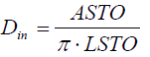
In order to handle complex structures, the storage or pipe mass MSTO, the heat exchanging area ASTO of the pipe side facing the fluid can be set by the user as well as the length of flow LSTO. The governing equations are:
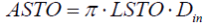 |
(1) |
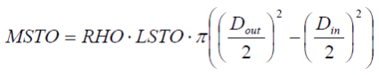 |
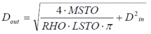
(2) |
whereas Dout and Din mean outer and inner diameters, RHO represents the density of the pipe/storage material. The resulting geometry of the pipes is defined:
 |
(3) |
 |
(4) |
The fluid containing volume is determined by the geometry of the pipe:
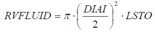 |
(5) |
or the specific value of VSTO can be chosen, what shows advantages in case of complex structures, which deviate from the pipe model. This provides a flexible approach for many modeling applications.
FSTO=1: via LSTO, DIAI and THSTO
Alternative it is possible to fix the geometry of the storage by defining the following parameters:
LSTO: Pipe length
DIAI: Inner diameter of the pipe
THSTO: Thickness of the pipe wall
An off-design pressure loss calculation based on the specific volume at the inlet of the component can lead to higher inaccuracies, if the temperature change between inlet and outlet is high and the flowing medium is compressible / gaseous.
This is why there is the FDPBASE switch, where the mean value of the specific volume between inlet and outlet can also be used and the nominal value V12N (the mean specific volume between inlet and outlet) can be used as a reference value.
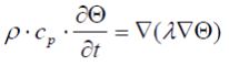
For a certain conductivity of temperature:
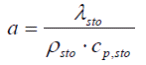 |
(6) |
and given distances dX and dY to the neighbour points, the distribution of temperatures Θ in the walls is calculated by solving the differential equation for all discrete elements in the storage:
 |
(7) |
simplified to two dimensions the yield is:
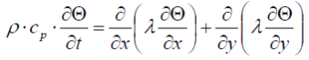 |
(8) |
Changes to the temperatures starting at an initial state always occur due to heat flow through the wall and the insulating surface (see also chapter 3).
For FALGINST=1 (2D-Grid Crank-Nicolson-Algorithm) the equation (8) is discretized and solved numerically. The number of grid elements in X direction (here the flow direction of fluid) can be manipulated by the user input value NFLOW. The number of grid elements in Y direction (here the direction normal to the tube wall) can be manipulated by the user input value NRAD. The numerical solution results in a 2-dimensional Temperature field in the storage wall. This resulting field can be observed in matrices MXTSTO, RXTSTO (see below).
For FALGINST=4 (model using combined analytical and numerical methods) only 1 grid element is used in wall normal direction Y. For each element there is a mean temperature which is searched for. The heat conductivity in the flow direction is neglected.
The storage temperature after the time step Dt can be computed as
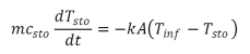 |
(8.1) |
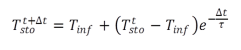 |
(8.2) |
As no temperature gradients occur within a discretisation element, this approach can be integrated directly and we receive the form of the solution for the storage temperature as a function of the time step width shown in Equation (8.2). The two temperatures with the index “sto“ describe the condition of the storage tank before and after the time interval Dt, here Tinf as a driving force describes the steady-state final temperature of the storage wall element, and t is the storage time constant mc/kA.
Heat flow between the walls and the fluids depends on position and time, what is described mathematically by linking the convective 9a to the conductive terms 9b:
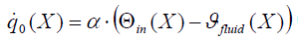 |
(9a) |
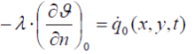 |
(9b) |
whereas  represents the temperature of the wall area facing the fluid.
  is the temperature of the media and
  indicates that the direction of the heat flow is orthogonal to the flow direction of the fluid. Heat flow at outer wall will be calculated equivalently.
Heat fluxes at the walls induce a change of the media temperatures, which also influences the whole 1-D grid of the fluid. Gradients orthogonal to the flow direction and the flow dynamics as well will be neglected in order to keep the model simple and save CPU-time. Calculation of time dependent changes of the temperatures will be done based on mass and energy balances for every volume element.
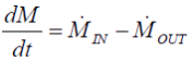 |
(10a) |
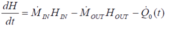 |
(10b) |
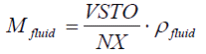
The enthalpy of a fluid element is given by 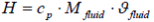 , introduced to eqn 10b the result is:
 |
(11) |
Left side of this equation shows the energy stored in the fluids, while the right side gives the resulting energy flows from the walls trough the boundaries. Mass of a fluid element is defined by:
 |
(12) |
All property calculations of the media are based on the EBSILON material properties.
Prior to Release 17, the numerical scheme for calculating the fluid temperatures was dependent on the FSPECM switch. For FSPECM=1 (fluid mass neglected), the CDS (central differences) scheme was always used. For FSPECM>1 (fluid mass taken into account) the upwind scheme was used.
The CDS scheme is more accurate than the upwind scheme. However, the upwind scheme is more stable for the internal convergence of the component.
From Release 17, the FNUMSC switch is available. This allows the user to select the numerical scheme independently of the FSPECM value. FNUMSC=0 corresponds to the upwind scheme, FNUMSC=1 corresponds to the CDS scheme.
If the inner iteration switches from CDS to Upwind due to detected convergence problems, the user is warned at the end of the simulation.
In the circuits saved with earlier EBSILON versions than Release 17, the value of the FNUMSC switch is set depending on the FSPECM switch when loading in order to reproduce the old results. However, this automatic setting of the switch does not work if FSPECM does not have a simple valid numerical value, but contains a reference (kernel expression) to other components, for example. In such a case, the user should set the FNUMSC switch himself so that the old results are reproduced.
FSPECM=1: In case of continuous flow Min = Mout conditions and neglectible fluid mass in comparison to the mass of the wall, left side of eqn 11 is set to zero, what simplifies the following calculation to:
 |
(13) |
FSPECM=2: In case of continuous flow Min = Mout or a zero mass flow Mfluid = 0, there´s no change of the masses in the duct pipe. But if the second condition concerning the mass ratio of fluid and storage and coupled to this the energy content of the fluid has to be taken into account, it´s necessary to chance eqn 11 to the following:
 |
(14) |
Example: Cooling down a stagnant thermo liquid in duct.
FSPECM=3: Fluid mass inside the pipe is variable, what can be the result of changing density as a function of pressure and temperature. In assumption of a constant duct volume different mass flows at inlet and outlet can occur. To define the thermodynamical state of the fluid in the beginning of the time series the specification values TAVSTART, HAVSTART and PAVSTART can be used.
Example: Evaporation from a vessel after a pressure drop.
FSPECM=4: Inlet and outlet mass flow need to be specified and don´t have to be equal. As a consequence the properties and also the fluid mass in the storage are changeable. The numerical grid is reduced to one point in flow direction (NX=1), different input will be ignored. Initial state of the fluid is given by TAVSTART, HAVSTART and PAVSTART, what also fixes the fluid mass in storage via the relation m = r(p,H) V.
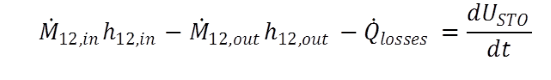
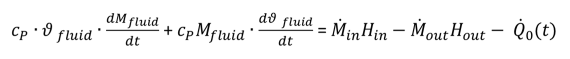
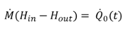
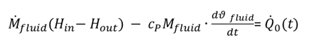
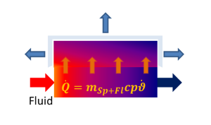
The calculation of the heat fluxes is done using eqn 11 combined with the settings given by switch FSPEM. In case of neglectible fluid mass the energy balance for both of the fluids appears as following:
 |
The mass of the storage, whose changes of temperature induces a heat flow (Q0(t)), only consists of the wall elements. The fluids are connected thermally via the following equation:
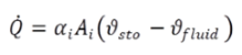 |
(15) |
In the same way the calculation of heat losses to the ambient (blue arrows) is carried out and passed to the result values of QAVO and QENDO. The transient storage behaviour is realized by solving the volume integral of all temperature changes:
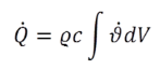 |
(16) |
Balancing all heat flows (according to eqn 2.13) delivers the stored amount of thermal energy with further integration concerning the time step. The result is passed to the variable QSTO:
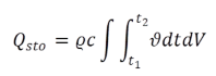 |
(17) |
This value QSTO divided by the interval of the time step Dt shows the mean heat flow QAV between wall and FLUID. While this heat flux changes time dependent, there´s a variable QEND representing the value at the end of the time step. To get a closed energy balance the amount of heat received from or given to the fluid is stored in the variables QAVI (mean value) and QENDI, which is also passed to line 3. The balance shows the following relations:
Tip: Dependent on the magnitude of the temperature gradients and the choice of the time step, it is not possible to get a closed energy balance. If greater miss balances appear, it will be reasonable to reduce the time interval or do a refinement of the time step by adjusting FTSTEPS.
If simulations are done with respect to the fluid mass (FSPECMXX = 2,3 and 4), balancing becomes different as shown below:
 |
Left side of eqn 2.8 is not zero anymore, hence fluid mass is considered in this equation. The walls and fluids as well are acting as transient energy storage.
When calculating a fluid at rest (e. g. standby mode of the storage tank), the heat conduction in the fluid must always be taken into account (FHC=1), whereas in the case of a flowing fluid in the storage tank neglecting the heat conduction in the fluid is justified (FHC=0).
For the heat exchange between the fluid elements in the storage tank, the material value tables of the fluid are used for the calculation of the thermal conductivity.
In addition, the thermal conductivity can be multiplied by a factor CLMFL. This may be necessary, for example, in the case of free convection in the storage tank.
In the beginning of a time series calculation the temperature profile has to be defined. This is done whenever the switch FINIT ist set to 1. According to switch FSTART there are two possibilities to get initial values for the storage temperature.
FSTART=1: The whole temperature profile is set to the value TSTART.
FSTART=2: A first calculation delivers the temperature distribution in the storage as a long
term asymptote using the specifications of ambient temperature, thickness of the
pipe, heat conductivity LAM, the heat transfer coefficients ALPHI and ALPHO.
The switch FINST generally controls the transient behaviour of the component.
FINST=0: Intervals of the time dependent calculation steps are given by the time series dialogue, which takes control of the whole calculation. All transient terms including thermal storages in the equations are going to be solved.
FINST=1: The calculation is always steady state. All fluid data will be passed directly to line 2 without any calculations.
FINST=2: An transient single calculation is done with the time step interval given by TIMESING. The simulation is started with the "Simulate" button.
FINST=3: An transient single calculation is done with the time step interval given by TIMEMAX from the model options panel (Simulation > Transient > Time handling > calculate maximum)
The simulation is started with the "Simulate" button.
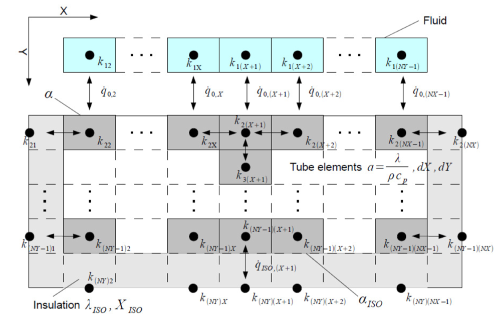
Figure 2: Internal numerical grid of the storage device
All transient components that possess the flag FINIT can be commonly controlled via one global flag.
For this, the flag FINIT has been expanded by the position GLOBAL: 0.
If it is set to this value, the control of the transient simulation will be handed over to the global variable “Transient mode“, which can be found under
Extras \Model Options\Simulation\Transient\ Combo Box "Transient mode".
This will then pass on the desired mode (first iteration or following iteration) to the components. This can be controlled from the time series dialog by means of the expression “@calcoptions.sim.transientmode“.
In order to set up temperature dependent material properties, three characteristics are introduced:
All plots showing the temperature on their X-axes.
All other "characteristic lines" form a circular buffer. The user doesn´t have to take care of them.
Corresponding to this "characteristic lines", there are also result arrays.
Specification matrix MXTSTO and result matrix RXTSTO
The matrix MXTSTO is linked to the result matrix RXTSTO in the same way as the characteristic curves and result arrays mentioned above.
The distribution of the values in the storage and the fluids is stored in both matrices (default matrix MXTSTO for time step t-1 and result matrix RXTSTO for time step t).
For the structure of the matrices, see matrices of component 119.
|
Form 1 |
Click here>> Component 119 Demo << to load an example.