Component 10: Feedwater Preheater/Heating Condenser

In This Topic

Component 10 : Feed Water Preheater / Heating Condenser

Specifications

Line connections
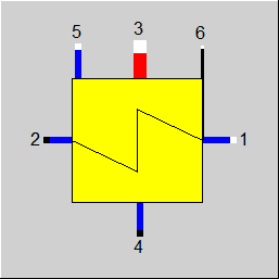
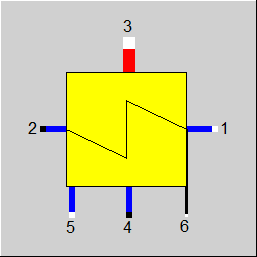
1	Inlet (cold medium, flows inside the tubes)
2	Outlet (cold medium, flows inside the tubes)
3	Inlet (hot medium, flows external to the tubes)
4	Outlet (hot medium, flows external to the tubes)
5	Auxiliary condensate inlet (without throttle)
6	Control inlet for KAN (as H)

General User Input Values Characteristic Lines Physics Used Displays Example

General

Component 10 can be used, when a gas (steam or superheated steam) is to be condensed to heat a cold medium (gas or liquid).
Typical application examples are the modeling of a

feed water preheater or a
Heating condenser for district heating.

Like most components, the component can be designed with a design calculation, i.e. nominal values are calculated, transferred and stored in a design calculation. Alternatively, it is also possible to completely describe the component by entering geometry and material data.

In this case a transient calculation is also possible, i.e. time-dependent heat input and output processes in the component material can be calculated.

In all calculation modes component 10 calculates the required steam quantity to be condensed for the respective specifications. If this steam quantity is specified from the outside, the condenser (component 7) or the heat consumer (component 35) can be used instead.

The component represents the desuperheating of the superheated steam and its condensation, but no sub cooling. The outgoing condensate is therefore basically saturated liquid. To model sub cooling, an after cooler (component 27) has to be added.

The cold medium is usually water, almost all other media can be used, e.g. for modeling a steam LUVO. The warm medium can be steam, two-phase fluid, binary mixture or a corresponding universal fluid.

Design

In case of design, FSPECD has to be set: Either

as upper terminal temperature difference DT3S2N (see heat exchanger in general), i.e. the temperature difference between the saturated steam temperature of the incoming steam and the outlet temperature of the heated cold medium. In the case of superheated steam, the cold medium can become hotter than the condensate. In this case the upper temperature difference must be specified negatively.
or as the outlet temperature of the heated cold medium from outside (i.e. not inside the component)

The result of the design calculation is, among other things, the nominal value for k*A, known as KAN. In the case of the geometry-based calculation (FGHXT=1), the NTU-Effectiveness correction factor CORCFN and the cleanliness factor CLTUBE are calculated in the design calculation.

k: overall heat transfer coefficient,
A: heat transfer surface,
k*A: heat transfer capability, product of k and A
KAN: Heat transfer capacity at the design point (nominal value)

The component can also be used with fluid type Binary fluid as warm fluid. If this fluid is overheated, the grade DT3S2N refers to the dew point temperature of the fluid (as for component 7), otherwise to the fluid temperature.

Radiation losses can be specified via a related loss factor. The switch FDQLR is used to set how DQLR (factor for modeling heat losses) should be interpreted. In a calculation with geometry, radiation losses are calculated from the parameters for the insulation (THISO, LAMISO), the external convective heat transfer coefficient ALPHO and the ambient temperature.

As a real heat exchanger, unlike the model component, is not a pure counter current heat exchanger, the calculation of the heat transfer is corrected with a cross-flow correction factor (value < 1). This factor is determined in the design calculation according to a stirred tank model (VDI-Wärmeatlas edition 11 chapter C1) and stored as nominal value CORCFN for the partial load calculation.

Partial load behaviour

The partial load behaviour is calculated with one of these methods:

via characteristic curves or
via a deposited formula (Rabek method)
from geometry data

Switching is done with the FRABEK and FGHXT switches.

In the case of superheated steam at the inlet, component 10 considers two zones: the desuperheating zone and the condensation zone. In both zones the heat transfer coefficients (alpha numbers) between the warm fluid and the tube wall are different. In no case is an analytical calculation method used.

The alpha number (Convective Heat Transfer Coefficient) for the condensation zone is named AL34N, the alpha number for the desuperheating zone is named AL34DN.

With FGHXT=1 the numerical
algorithm from component 126 is used, which is based on the specification of the complete geometry data.
The following are taken into account

- The heat transfer between the cold fluid (12) and the tube wall
- The heat transfer between the warm fluid (34) and the tube wall
- The heat transfer between the warm fluid (34) and the jacket wall
- The temperature curve in the pipe wall
- The temperature curve in the jacket wall

For the calculation of the convective heat transfer coefficients (AL12, AL34) there is a choice between the formulas available in the VDI Wärmeatlas and your own data, e.g. in the form of a function specified by the user (EALPH12, EALPH34). The user can specify the value AL34DN as constant and additionally scale it at partial load with a mass flow exponent EX34D.
With FGHXT=0 and FRABEK = "No" a partial load value for k*A from KAN is determined by multiplication with the scaling factors resulting from the two characteristic curves CKAM1 and CKAM2. This simplified method assumes that the separation zone between the heating part and the condensing part is fixed and does not shift in partial load mode. This method can cause pinch point problems at very low loads (below 50%) (the temperature gradients become too small).
With FGHXT=0 and FRABEK = "Yes" the partial load behaviour is determined according to the method of Rabek. This method offers the advantage, especially in case of superheated steam, that a shift of super heating and condensation zone is taken into account depending on the load case. This method was published in the sixties by Prof. Rabek and takes into account a movement of the separation zone. This method corresponds more to reality, but is much more complex in the calculation.

Identification mode (OFf Design only)

Similar to other components, a FIDENT switch has been introduced to activate the identification mode.
FIDENT has the settings:

0: no identification
2: Identification or calculation of k*A by specifying T2, the outlet temperature of the cold current, given externally in partial load
-11: Only consideration of mass and energy balances and H4 = H'
11: consideration of mass and energy balances and Fourier equation LMTD * KAN - M1*(H2-H1) = 0

FIDENT =-11 and FIDENT =11 were made accessible for special data reconciliation requirements, which corresponded to the previous settings, under FSPEC=-11 and FSPEC =11 respectively.

In order not to change the behaviour of existing models, the switch FSPEC can still be used. In this case the settings for FIDENT and FSPECD are ignored.

Note in connection with the Rabek method:
Since this method is non-linear, when using quality grades as correction factors, a correction factor determined in part load cannot simply be used to correct the nominal values. EBSILON®Professional provides the result value KANRAB for this purpose. This is the fictitious value for KAN, which in a partial load calculation without identification mode would lead to the result obtained in identification mode.

Transient modeling

Component 10 enables the modeling of transient cases (time-dependent temperature distribution). This type of calculation is activated with the switch FINST. A thermodynamic equilibrium between the liquid and the gaseous phase in the condensate space is assumed.

For the transient calculation, the specification of the geometrical details of the heat exchanger is necessary, such as the geometrical and material specifications of the casing or jacket. For this purpose the switch FGHXT=1 is used. From the geometrical data the fluid volume, the wall storage mass and the exchange surface between wall and fluid are calculated. The properties of the wall material such as density, thermal conductivity, heat capacity can either be selected from the stored library (switch FMTUBE, FMSHELL) or directly specified by the user.
With FGHXT=1 the heat transfer is calculated also in stationary case with geometry.

For the stationary solution of heat exchange with FGHXT=1 (geometry based) component 10 uses the numerical algorithm, because no simple analytical relation between K-number and alpha-numbers in case of 2-zones (desuperheating and condensation) is possible. With this numerical algorithm the result depends on the number of points in the direction of flow (NFLOW).

The transient mass balance takes into account a level change in the condensate space during the time step. For the mass balance, the user can use the FSPIN switch to decide between setting the level or the mass flow M4. The calculated level is output as the volume fraction of the liquid phase in the volume between the values of VMIN and VMAX at port 6 as mass flow M6.

Specification of component properties from outside

(see also: Edit objects --> Connections)

To make component properties such as efficiencies or heat transfer coefficients (variation quantity) accessible from the outside (for control or validation) it is possible to place the corresponding value as indexed measured value (default value FIND) on an auxiliary line. The same index must then be entered in the component as default value IPS.

It is also possible to place this value on a logic line at connection 6, which is directly connected to the component (see FVALKA=2, variation size: KAN, dimension: enthalpy). The advantage is that the assignment is now graphically visible and thus errors (for example by copying) are avoided.

Note about result values

Grade RPFHX

For the assessment of the condition of component 10 the quotient of the current value for k*A (result value KA) and the k*A expected at the respective load point due to the component physics or characteristics (result value KACL) is used. The quotient KA/KACL is output in the result value RPFHX.

If the RABEK method is used, the quotient KANRAB/KAN is displayed in RPFHX instead.

For further general information with reference to most common heat exchangers see Heat Exchangers, General Remarks

For more information on comparing this heat exchanger with other heat exchangers, see Heat Exchangers, General Components

User Input Values

FINST	Transient mode: 0: Transient solution (time series or single calculation) 1: Always steady state solution
FMODE	Flag for calculation mode design/off-design =0: global =1: local off-design (i.e. always off-design mode, even when a design calculation has been done globally) =2: special local off-design (special case for compatibility with earlier Ebsilon-versions, not to be used in new models, because the results of the real off-design calculations are not consistent) = -1: local design
FFU	Flag for activating the component = 1: Heat exchanger switched on = 0: No heating of the cold steam. In this mode only a heating of the feed water is prevented. However, the condensate outlet is still kept at saturated water conditions. When super-cooled auxiliary condensate is fed, then only so much steam is extracted that this can be warmed to the saturated water temperature. =-1: The steam supply is completely stopped. When super cooled auxiliary condensate is supplied, then this comes out as super cooled too. The pressure drop for the cold side is treated the same way in all cases.
FIDENT	Component identification =0: NO Identification =2: T2 (outlet temperature of cold stream) given externally in off-design, KA calculated =-11: Consider mass and energy balances and H4=H' only =11: Consider mass and energy balances and Fourier equation LMTDKAN-M1(H2-H1)=0
FSPECD	Design specification method =0: Design using DT3S2N =1: Design using T2 (given externally)
DT3S2N	Upper terminal temperature difference T3S-T2 (Default only in design case)
FDP12	Cold side pressure drop handling =1: Calculation of the pressure loss from the nominal value DP12N =-1: P2 Pressure specification from outside
DP12N	Cold side pressure drop, line 1 to 2 (nominal)
FDP34	Hot side pressure drop handling =1: Calculation of the pressure loss from the nominal value DP34N =-1: P4 Pressure specification from outside
DP34N	Warm side pressure drop, line 3 to 4 (nominal)
FDPNUM	Pressure loss handling in the numerical solution =0: Using the average fluid pressure between inlet and outlet =1: Use of a linear pressure distribution between inlet and outlet, corresponding pressure values in the individual NFLOW fluid elements
FP5	Throttling of secondary condensate =0: No throttling (P5 = P3) =1: Throttling at pin 5 - (P5 given externally)
FDQLR	Heat loss handling =0: Constant (DQLRQN in all load cases) DQLR refers to the design value QN (which equals the heat quantity given off by the hot flow in the design case) in all load cases, i.e. it has a constant value in all load cases. If, however, this value exceeds 10 percent of the heat quantity given off by the hot flow, the heat loss will be limited to this value, and a warning will be output. =1: Relative to actual heat input (DQLRQ354) DQLR refers to the heat quantity given off by the hot flow. If the corresponding warning is ignored, losses of more than 10 percent can be modelled here too.
DQLR	Relative heat loss to the environment
TOL	Accuracy of the energy balance for the internal iteration
FRABEK	Calculation according to the method of Rabek =0: No (instead, using the characteristic lines) =1: Yes (Characteristic lines are ignored)
FFLOW	Direction of flow =0: (currently not used)
FSPEC (deprecated)	Deprecated specification combi switch =-999: unused (FSPECD and FIDENT used instead) Deprecated values: =0: Outlet temperature T2 calculated (in design from DT3S2N, in off-design using Fourier's law) This is the normal calculation mode of the component. =5: Outlet temperature T2 specified externally in design, calculated in off-design =-1: Outlet temperature T2 specified externally in all load cases (constant) (identification mode) =-11: Consider mass and energy balances and H4 = H' only. Note: If this method is used in off-design, the mass and energy balances will be observed, but the heat exchanger will be resized. Use this method only when appropriate, such as for data reconciliation. This method could violate the second law of thermodynamics. =11: Consider mass and energy balances and Fourier Equation LMTD * KAN - M1*(H2-H1) = 0
FADAPT	Flag for using the adaptation polynomial / adaptation function =0: Off =1: Correction factor for kA [KA = KAN carlines factor polynomial] =2: Calculation of kA [KA = KA * polynomial] =1000: Not used but ADAPT evaluated as RADAPT (Reduction of the computing time) =-1: Correction factor for kA [KA = KAN carlines factor function] =-2: Calculation of kA [KA = KA * function] =-1000: Not used but EADAPT evaluated as RADAPT (Reduction of the computing time)
EADAPT	Adaptation function for KA
FVALKA	Validation of k* =0: KAN used without validation =1: Pseudo measurement point identified by IPS used (can be validated) =2: KAN given by enthalpy on logic line 6
IPS	Index for pseudo measurement point
KAN	k*A (nominal) - Design Heat Transfer Capability
M1N	Cold side mass flow (nominal)
M3N	Hot side mass flow (nominal)
V1N	Cold side specific volume (nominal)
V3N	Hot side specific volume (nominal)
QN	Heat quantity given off at nominal load (nominal)
CORCFN	NTU-Effectiveness correction factor (re-computed in design only)
FGHXT	Use geometry based approach (e.g. HEI, VDI) in heat transfer calculation 0: No 1: Use Alpha and Lambda values according to FALPH and FMTUBE
FTUBG	Tube geometry specification (HEI, transient calc.) 0: Use DTUBEIN and DTUBEOU 1: Use DTUBEIN and DWALL 2: Use DTUBEOU and DWALL
DWALL	Tube wall thickness
DTUBEIN	Inner diameter of tube
DTUBEOU	Outer diameter of tube
FBUNDL	Tube bundle specification 0: Use NTUBE, NPASS and ATUBE 1: Use NTUBE, NPASS and TUBELEN
NTUBE	Number of tubes
NPASS	Number of tube passes
ATUBE	Total outside tube surface area
TUBELEN	Tube length
SDIAM	Shell diameter
SLENG	Shell length
SWALLT	Shell wall thickness
THISO	Thickness of insulation
CLTUBE	Cleanliness factor
FINIT	Flag: Initializing state =0: Global, which is controlled via global variable "Transient mode" under Model Options "Extras" ->"Model Options" -> "Simulation" -> "Transient" -> Combo Box "Transient mode" (See -> Used Physics / equations -> Global Initialization of Transient Components ) =1: First run -> Initializing while calculating steady state values =2: Continuation run -> Values from previous time step are input for the present ones
FMTUBE	Steel grade for the tubes see Material Properties of Steel =-1 : Properties computed from kernel expression ERHOT, ELAMT, ECPT
ERHOT	Function for tube material density
ELAMT	Function for tube material heat conductivity
ECPT	Function for tube material heat capacity
FMSHELL	Steel grade for the shell see Material Properties of Steel =-1 : Properties computed from kernel expression ERHOS, ELAMS, ECPS
ERHOS	Function for shell material density
ELAMS	Function for shell material heat conductivity
ECPS	Function for shell material heat capacity
LAMISO	Thermal conductivity insulation
FALPH12	Determination of alpha fluid12 to wall 0: Using internal formulas from VDI Wärmeatlas Edition 11 Chapter G1 1: from constant value AL12N 2: from kernel expression EALPH12
AL12N	Cold side heat transfer coefficient (nom.)
EALPH12	Function for ALPH12
FALPH34D	Determination of AL34D 0: from constant value AL34DN 1: from AL34DN and flow rate exponent EX34D
AL34DN	Heat transfer coefficient desuperheating zone
EX34D	Flow rate exponent of AL34D
FALPH34	Determination of alpha fluid34 to wall 0: Using internal formulas from VDI Wärmeatlas Edition 11 Chapter J1 1: from constant value AL34N 2: from kernel expression EALPH34
AL34N	Hot side heat transfer coefficient (nom.)
EALPH34	Function for ALPH34
FALPHO	Determination of alpha outside 0: from specification value ALPHO 1: from function EALPHO
ALPHO	Outer heat transfer coefficient (to ambient)
EALPHO	Function for alpha outside
FSPIN	Transient balance calculation mode 0: Liquid level given, mass flows computed 1: Mass flows given, liquid level computed
VF	Averaged liquid volume fraction (liquid level) during the time step
VMIN	Volume at liquid volume fraction 0
VMAX	Volume at liquid volume fraction 1
FLVCALC	Liquid volume calculation mode 0: linear between VMIN and VMAX 1: Using ELV
ELV	Function for the liquid volume computation
NFLOW	Number of points in flow direction (max. 100)
FNUMSC	Numeric scheme 0: Upwind (highest stability) 1: Central differences (high accuracy)
TMIN	Lower limit for storage temperature
TMAX	Upper limit for storage temperature
FSTAMB	Definition of ambient temperature 0: by specification value TAMB 1: defined by reference temperature (comp. 46)
TAMB	Ambient temperature

The parameters marked in blue are reference quantities for the off-design mode. The actual off-design values refer to these quantities in the equations used .

Generally, all inputs that are visible are required. But, often default values are provided.

For more information on colour of the input fields and their descriptions see Edit Component\Specification values

For more information on design vs. off-design and nominal values see General\Accept Nominal values

Result values

Q21	Heat quantity, by which the cold stream (line 1 to line 2) is heated
QT	Heat quantity calculated from the product of KA * logarithmic temperature difference
QT354	Heat quantity, which is extracted from the main and auxiliary condensate (sum from line 3 and 5 after line 4) The values of Q21, QT and QT354 should match in their calculation efficiency. Differences indicate errors or inadequate convergence.
KA	Heat transfer coefficient * area
KANR	Used value for KAN
KANRAB	Fictitious value for the nominal value KAN, which would lead to the value for k*A when the Rabek-method is used, which is currently set (owing to temperature specifications). This value helps in determining the quality grade of the component from the measurement values. Owing to the non-linearity of the Rabek-formalism this cannot be done simply from the ratio of KA/KACL, but instead it must be determined through a reverse calculation of the Rabek-formula of the value for KAN, which leads to KA through the measured values in the actual load case. KANRAB is calculated only when the component is present in the identification mode (FSPEC = "fixed specification of outlet temperature" or FSPEC = "outlet temperature can be validated"), FRABEK was set to "Yes", present at the hot inlet of superheated steam.
RPFHX	Performance factor Heat transfer
DTM	Average logarithmic temperature difference. In the counter current mode (which is always the case in this component): DTM = ((T3S-T2)-(T4S-T1)) / LN ((T3S-T2)/(T4S-T1)) Thereby, T3S and T4S are the saturation temperatures for the pressures P3 and P4 respectively. Since in the calculation method according to Rabek negative terminal temperature differences can occur, in this case an effective DTM is output from the quotients of the exchanged heat quantity and k*A.
DT4S1	Lower terminal temperature difference In the counter current mode (which is always the case in this component): DT4S1 = T4S-T1
DT3S2	Upper terminal temperature difference In the counter current mode (which is always the case in this component): DT3S2 = T3S-T2
X1	Steam quality (cold side outlet) (pin 2). For reasons of compatibility with the DOS-version this value was still retained as result value, meanwhile the steam content is also accessible at the line or via $._2.X.
X2	Steam quality (hot side outlet) (pin 4). For reasons of compatibility with the DOS-version this value was still retained as result value, meanwhile the steam content is also accessible at the line or via $._4.X.
DP12	Calculated cold side pressure difference DP12 = P1 - P2
DP34	Calculated hot side pressure difference DP34 = P3 - P4
M1M1N	Ratio of the actual cold side mass flow to its nominal value: M1M1N = M1 / M1N
M3M3N	Ratio of the actual hot side mass flow to its nominal value: M3M3N = M3 / M3N
KAKAN	Ratio of the actual k*A to its nominal value: KAKAN = KA / KAN
KACL	Fictitious value of k*A, which would result, if the calculation was done only with characteristic lines: No identification mode, but instead FSPEC = "Outlet temperature T2 calculated" No Rabek-method, but instead FRABEK = "No" No adaptation polynomial, but instead FADAPT = "Not used" KACL is the same as the product of KAN and both the factors from the 1/2 and the 3/4 KA-characteristic lines.
RADAPT	Value of the adaptation polynomial used This value is calculated only when the adaptation polynomial is used; else it is 1.
PINP	Pinch point The pinch point is defined as the temperature difference at the transition point between deheating zone and the condensation zone: PINP = T3S - TP whereby TP is the temperature of the primary medium, which is set when one adds only the heat of condensation to the primary medium (i.e. without the heat from deheating). The following is true: HP = H1 + ((H(T3S)-H4)/(H3-H4)) * (H2-H1) TP is then the temperature calculated from HP and P2 with the water-steam table.
HSAT	Hot side saturated steam enthalpy
TSAT	Hot side saturation steam temperature
PSAT	Hot side saturation steam pressure
SSAT	Hot side saturated steam entropy

Characteristic Lines

1^st Characteristic Line CKAM1 FK1 = f (M1/M1N)

2^nd Characteristic Line CKAM3 FK2 = f (M3/M3N)

(K*A)/(K*A)N = FK1 * FK2

Characteristic line1: (k*A)-Characteristic line CKAM1 : (k*A)1/(k*A)N = f (M1/M1N)

     X-Axis    1        M1/M1N                         1^st point
                    2        M1/M1N                         2^nd point
                    .
                    N        M1/M1N                        last point
    Y-Axis    1        (k*A)1/(k*A)N                  1^st point
                    2        (k*A)1/(k*A)N                  2^nd point
                    .
                    N        (k*A)1/(k*A)N                 last point

Characteristic line 2: (k*A)-Characteristic line CKAM3: (k*A)2/(k*A)N = f (M3/M3N)

     X-Axis      1        M3/M3N                         1^st point
                    2        M3/M3N                        2^nd point
                    .
                    N        M3/M3N                        last point
    Y-Axis      1        (k*A)2/(k*A)N                 1^st point
                    2        (k*A)2/(k*A)N                 2^nd point
                    .
                    N        (k*A)2/(k*A)N                 last point

Physics Used

Design case (Simulation flag: GLOBAL = design case and FMODE = GLOBAL)

T3S = f'(P3)

P2 = P1 - DP12N

T2 = T3S DT3S2

H2 = f(P2,T2)

M2 = M1

Q2 = M2 * H2

DQ = M2 * H2 - M1 * H1

P4 = P3 - DP34N

P4 = P5

Q4 = Q3 + Q5 - DQ/(1-DQLR)

M4 = M3 + M5

H4 = Q4/M4

T4 = f(P4,H4)

DTL = T4 - T1

DTU = T3 - T2

LMTD = (DTU - DTL)/(ln(DTU) - ln(DTL))
(k*A) = DQ/LMTD

M3 = (DQ/(1-DQLR)-M5*(H5-H4S))/(H3-H4S)

Off-design case (Simulation flag: GLOBAL = off-design or FMODE = local off-design)

F1 = (M1/M1N) ** 2

P2 = P1 - DP12N * F1

M2 = M1

Fk1 =f(M1/M1N) from characteristic line 1

Fk2 =f(M3/M3N) from characteristic line 2

(k*A) = (k*A)N * Fk1 * Fk2

F3 = (M3/M3N) ** 2

P4 = P3 - DP34N * F3

P4 = P5

M4 = M3 + M5

Pre-estimation before beginning the iteration

T4 = f'(P4)

H4 = f'(P4)

H2max = f(P2,T3)

Q12max = M1 * (H2max - H1)

Q34max = Q3 + Q5 - M4 * H4

Qmax = min(Q12max,Q34max)

Q12 = 0.5* Qmax

Start of iteration

H2 = H1 - Q12/M2

T2 = f (P2,H2)

DTL = T4 - T1

DTU = T3 - T2

LMTD = (DTU - DTL)/(ln(DTU) - ln(DTL))

QQ = (k*A) * LMTD

DQQ = Q12 QQ

Start of the Regula Falsi method
grad = (Q12 - Q12old)/(DQQ - DQQold)

Q12 = Q12 - DQQ * grad

End of the Regula Falsi method

DQ = | DQQ/((Q12+QQ)/2.0) |

If DQ < TOL, then end of iteration
else continue the iteration

M3=(Q12+QN*DQLR-M5*(H5-H4) )/(H3-H4)

Q4 = M4 * H4

Q12 = (Q3 + Q5 - Q4 - QN*DQLR)

Q2 = Q1 + Q12

H2 = Q2 / M2

T2 = f (P2,H2)

DQ = M2 * H2 - M1 * H1

Component Displays

	Display Option 1
	Display Option 2

Example

Click here >> Component 10 Demo << to load an example.

Settings

Preheater - using Rabek's method

Impressum Disclaimer