
EBSILON®Professional Online Documentation


|
Line connections |
|
|
|
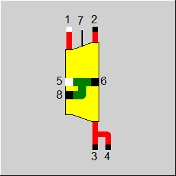
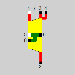
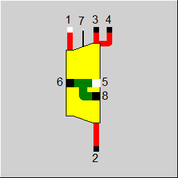
1 |
Steam Inlet |
|
|
2 |
Steam Outlet |
|
|
3 |
Extraction 1 |
|
|
4 |
Extraction 2 Steam /"NONE" |
|
|
5 (8) |
Shaft inlet Shaft / "NONE" If shaft inlet 5 should be active, then that is |
|
|
6 |
Shaft outlet |
|
|
7 |
Control inlet for efficiency (as H) Control inlet / NONE |
|
|
8 |
Shaft outlet Shaft / "NONE" If shaft outlet 8 should be active, then that is |
|
General Shaft connection Calculation Total vs Static Isentropic Efficiency User Input Values Characteristic Lines Physics Used Displays Results Displays Example
Component 6 serves the purpose of converting thermal/potential energy of a process stream into mechanical energy to a shaft. It can be applied to water (incompressible flow, hydraulic turbine), to steam or any other gases as defined by stream type Gas, Flue Gas, Universal Fluid, and 2-phase vapor/liquid ( compressible flow, turbo machinery). As such it is a most versatile component in EBSILON to model energy conversion by means of expansion of a process stream.
Component 6 represents a single expansion stage, a stage group, or a complete expansion section of the modelled equipment. Any extraction or admission along the expansion process must be modelled using multiple instances of component 6. Admission must be added by means of a mixer into the connecting process stream between two adjacent components 6. Extraction streams can be modelled, using any or both of ports 3 and 4, which have been added for convenience to spare addition of a splitter.
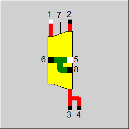
In the past, the second shaft connection on component 6 (steam turbine) was a shaft input. This made it possible to connect several turbine discs in series for component 6, so that the shaft power was added together.
The reverse case of power splitting for component 6 could not be represented graphically in the past. However, there was a switch FQ (power flow) for the calculation, with which the calculation could be changed, but with the drawback that the graphical representation then did not match the calculation.
The reverse power flow can now also be displayed graphically. Shaft connection 8 should be used for this.
To enable a corresponding visualisation, the previously existing connection has been hidden and the new connection has been positioned in the same place. Usually, either the input or the output is used and the unused connection should then be hidden. In principle, however, the software also allows both connections to be used simultaneously.
As with the previous second shaft connection, the power must also be specified on the new connection. The turbine can only calculate the power at the main shaft output.
The new connection means that the FQ switch is now superfluous. However, it is still available for compatibility reasons, but has been labelled as ‘obsolete’.
In addition, a comment message may be displayed to indicate the possibility of using the new connection. The switch also reverses the calculation direction for the new shaft connection.
A new result value QSHAFT has been implemented for component 6 (also for component 23, 58), which outputs the shaft power generated in the component, regardless of which connections it is distributed to or which shaft power is added.
CalculationThe calculation of the steam turbine has two objectives: the determination of (1) the flow characteristics which describe the correlation of throughput and inlet pressure, and (2) the power output which is determined as shaft power by means of an efficiency model.
The flow characteristic (inlet pressure as function of mass flow) is determined according to Stodola's law, which in essence means that the flow coefficient at the inlet, defined by
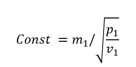
is constant for all operating modes. With m1 = inlet flow, p1 = inlet pressure and v1 = inlet specific volume.
In design mode, CF will be established using the inputs for flow pressure and specific volume. The user has two choices to specify the inlet pressure:
The outlet pressure P2 is always defined by external components. An external component can be the next expansion stage, a condenser, or a direct input be means of component 33 of 46.
At partial load, component 6 calculates the inlet pressure p1 as a function of the mass flow, outlet pressure and its specific volume from the Stodola law:
See also and for the formulation of the Stodola law: Turbines - OffDesign - Stodola
In the chapter "Part load calculation of the steam turbine", M1N, P1N, P2N and V1N designate the nominal values in the design case or M1, P1, P2 and V1 the corresponding quantities under the current conditions. As in the design case, the outlet pressure P2 is always determined by external components.
Component 6 uses an isentropic efficiency model to calculate the enthalpy drop during the expansion.
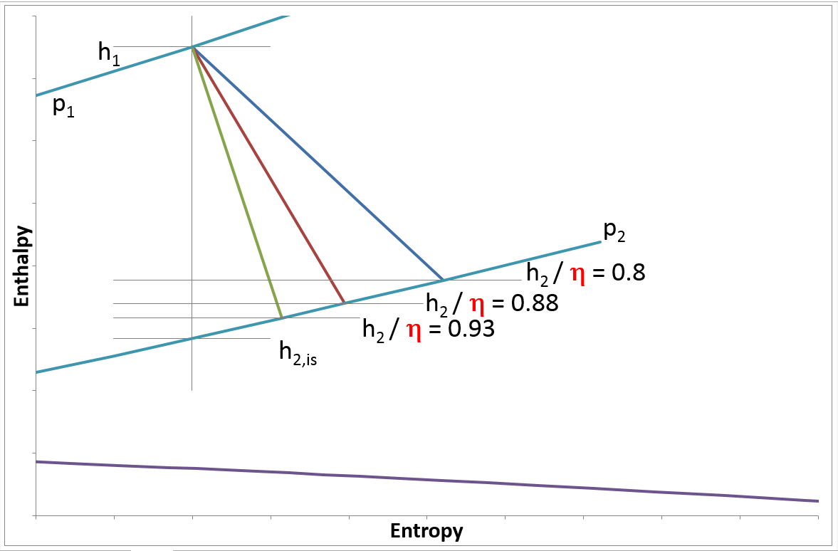
Figure 1: Enthalpy-entropy diagram of a simple expansion stage
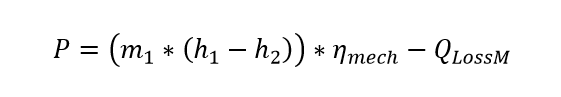
The mechanical energy output at the shaft evaluates as follows:
Using isentropic efficiency this converts to:
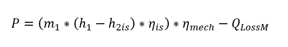
With m1 = inlet flow, h1 and h2 = inlet and outlet enthalpy, ηis = isentropic efficiency and mechanical losses as defined by QlossM in absolute terms or ηmech in relative terms. In design mode the user specifies exit enthalpy either directly by setting it outside component 6 on the exit stream by means of components 33 or 46 or by direct input of the isentropic efficiency with the parameter ETAIN. The off-design mode estimates the off-design efficiency relative to the nominal efficiency by means of correction curves (characteristic lines), which correlate the change of efficiency with the ratio of mass flow rate, or the ratio of volumetric flow rate, or the of change expansion pressure ratio.
Previously, identification modes of the steam turbine could be activated by a negative value of the flag for the characteristic line type (FCHR). This, however, is not just difficult to find for the user but also has the disadvantage that when determining the result value ETACL is is unknown which characteristic line type should be used. Previously ETACL was calculated for the characteristic line type FCHR=0 (mass flow-dependent characteristic line) for historical reasons.
Analogous to other components, a flag FIDENT has now been implemented also for the steam turbine. It has the following settings:
To prevent the behaviour of existing models from changing, the identification modes can still be activated by negative FCHR settings. In this case, the FIDENT setting is ignored. You will be notified by a comment.
When using FIDENT, the characteristic line type set in FCHR is now used for calculating ETACL.
It is possible to calculate the required steam mass flow for an externally given shaft power. This allows to directly model a feed water pump with power turbine. A controller had to be used to harmonize the required power of the pump with the turbine output.
This mode of calculation is activated by setting the new flag FSPECQ to 1. However, it can only be used for a single turbine disk. If several turbines and extractions exist, a controller has to be used for setting a required power output.
It is important to note that in EBSILON property calls are conducted without any reference to the flow velocity of the process streams, consequently all stream properties are based upon the total or stagnation enthalpies. The underlying convention is that EBSILON works on basis of total enthalpies.
The energy balance of turbo machinery can only be closed precisely and physically correct on basis of the total enthalpy values, unless exact knowledge of the flow velocities and inlet and exit swirls exists. Total and static enthalpies of a process stream correlate as follows:
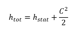
Figure 2 shows the corresponding expansion line in the enthalpy-entropy diagram, exactly relating static and total properties by the portion of kinetic energy.
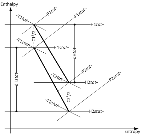
Figure 2: Total and static properties in the enthalpy-Entropy diagram for component 6
Isentropic efficiencies must be build consistently using either static or total properties.
In EBSILON applications for performance monitoring, where calculations are correlated with actual plant measurements, it is important to recognize that pressure and temperature measurements are rarely available in form of total pressure and total temperature measurements but rather in terms of static pressure and static temperature measurements. To be precise, these static measurements would need to be converted into stagnation properties, using above relationship. Figure 3 shows a balance, using the exact relationships, with total (stagnation) properties on the streams.
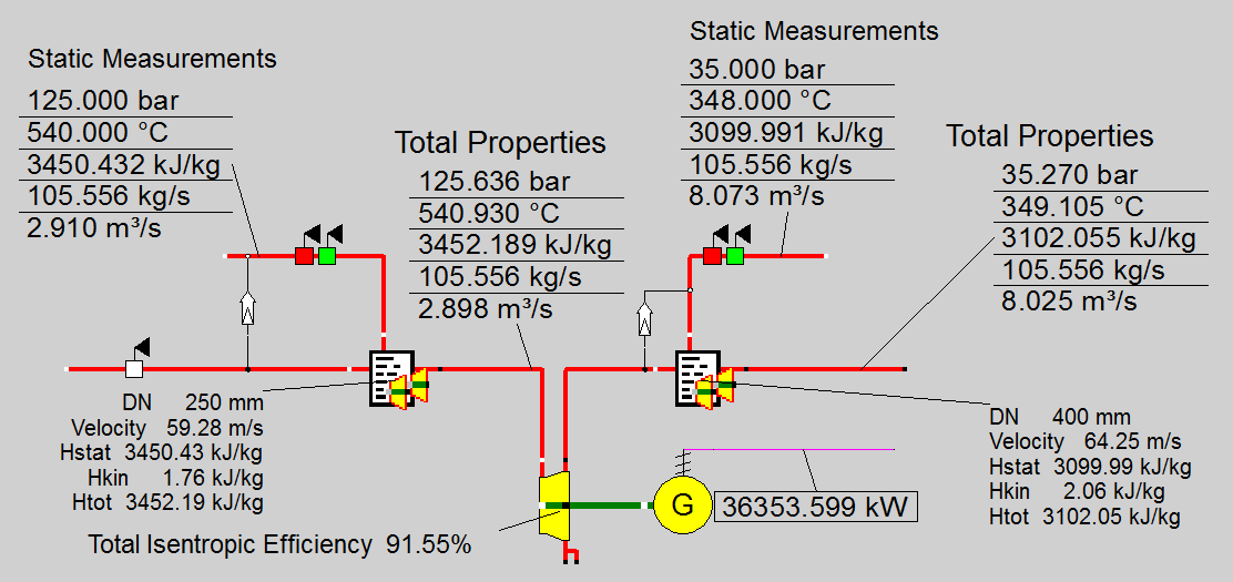
Figure 3: Energy balance around component 6, using correct definition of static vs total properties.
Yet, exact information about flow velocities at the point of measurement is rarely available. For practical purposes, these static measurements are frequently used directly to evaluate enthalpies for input into EBSILON. Figure 4 shows the same balance, using static measurements in lieu of total properties, feeding into component 6.
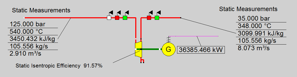
Figure 4: Energy balance around component 6, using static measurements.
The impact is small - in particular in relation to the absolute number - in regular applications where Component 6 is used to evaluate stage group efficiencies rather than at stage by stage expansion calculations. Typical design values for flow velocities in steam pipes and steam turbine intake and outlet structures are in the range of 50 to 70 m/s. This is roughly the same for inlet and outlet structures as indicated by significantly larger outlet flanges compared to the diameter of the inlet flanges.
The impact, whether performance is evaluated based upon static or total values is quite small in numeric terms. The uncertainty of pressure and temperature measurement is most of the time bigger than this ambiguity. Figure 5 shows an Enthalpy-Entropy diagram with expansion lines for both, one based on total properties and one based on static properties in true proportions. This clearly shows that the order of magnitude of the effects is negligibly small.
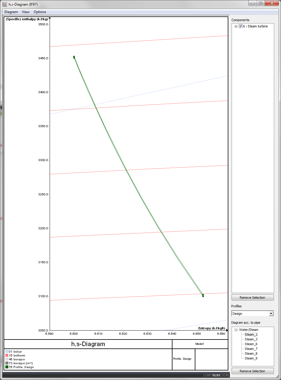
Figure 5: Enthalpy-Entropy diagram showing expansion lines based upon static and total properties in true proportions.
The enthalpy drop in above example, using static properties, evaluates to 350.442 kJ/kg, while the enthalpy drop, using total properties, evaluates to 350.135 kJ/kg a difference of less than 1/10 of a percent.
Nevertheless, EBSILON offers the user to account for effect of kinetic energy content by using the specification FSPEC= Total Isentropic Efficiency ,
CKIN1 and CKIN2' (FSPEC = 1). Figure 6 shows an energy balance around component 6, using the “Total Isentropic Efficiency” method.
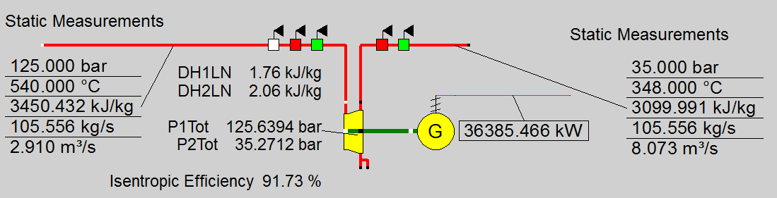
Figure 6: Energy balance around component 6, using static properties and total isentropic efficiency method.
Particular care must be taken if component 6 was to be used as the last stage before a condenser. At this position steam velocities leaving the expansion stage are in the order of 100 to 260 m/s, in some part load cases even up to sonic velocity, which is in the order of 410 m/s for steam, with associated kinetic energies ranging from 5 to 80 kJ/kg. In such case the kinematic component of the enthalpy cannot be neglected, particularly since its energy cannot be recovered by the turbine. It has to be considered as exhaust loss, which is dissipated to the environment through the condenser.
If enough information was available from DCS data, the user might want to reverse-engineer the efficiency characteristics of a particular expansion turbine. In such case, the user is advised to switch to component 122 for the task of modeling the condensing section. Component 122 uses industry standards for properly correcting expansion efficiencies for expansion into the wet steam region and to account for exhaust and ventilation losses. In addition, component 122 would also limit last stage expansion to Mach number equal 1, which actually constitutes a physical limit of steam turbine expansion in the last stage.
Polytropic efficiency
The FETA switch can be used to switch between isentropic (ETAIN) and polytropic (ETAPN) efficiency. Both (ETAI and ETAP) are calculated as the result value.
Switching to external presetting of efficiency on logic port 7 with switch FVALETAI was possible only when using isentropic efficiency (FETA=0). Now the external presetting is also applied to the polytropic efficiency (with FETA=1).
Since the calculation of the polytropic efficiency ETAP is very time-consuming (in some cases with complex material data, this multiplies the total calculation time of the model), the result value ETAP is no longer calculated automatically for each simulation. As was already the case with the compressor (component 24), the FOUTETAP switch has now also been introduced for component 6, with which it is possible to set whether ETAP should be calculated or not.
Logic inlet (Connection point 7) for controlling component properties
(see also : Editing components --> Ports)
To make component properties like efficiencies or heat transfer coefficients (variation quantity) accessible from the outside (for control or reconciliation) it is possible to place the respective value on an auxiliary line as an indexed measured value (specification value FIND). In the component, the same index must then be entered as specification value IPS.
It is also possible to place this value on a logic line that is directly connected to the component (please see FVALETAI=2, Variation variable: ETAIN, Dimension: Enthalpy). The advantage is that the allocation is graphically visible, and errors (e.g. when copying) are thus avoided.
The activation of this logic line can also be made conditional on the mode of calculation. This way, this feature can also be used for designs without having to switch manually all the time.
For this, the flag FVALETAI features the settings
This option is available for Components 2, 6, 8, 13, 18, 19, 23, 24, and 94.
In the case of the heat exchangers these setting options are unnecessary as using the logic line for specifying KAN is only possible in off-design calculations anyway. In design mode, KAN is calculated by Ebsilon, of course.
If connection point 7 is not used for efficiency specification but is available, the efficiency is output there as enthalpy. Depending on FETA, the isentropic efficiency ETAIN or the polytropic efficiency ETAPN is output.
|
FP1N |
Flag for the type of pressure definition Like in Parent Profile (Sub profile option only) Expression =0: P1 calculated from P1NSET (by Stodola equation) =1: P1-given from outside |
|
P1NSET |
Inlet pressure (nominal) |
|
FIDENT |
Component identification Expression =0: No identification |
|
FETA |
Efficiency type Like in Parent Profile (Sub profile option only) Expression =0: Isentropic efficiency =1: Polytropic efficiency |
|
FVALETAI |
Validation of the isentropic efficiency Like in Parent Profile (Sub profile option only) Expression =0: ETAIN / ETAPN used without validation =1: (Deprecated) IPS used instead of ETAIN / ETAPN(can be validated) =2: ETAIN / ETAPN given by enthalpy on control inlet 7 (enthalpy) =4: Enthalpy on control inlet 7 used in design, specification value ETAIN / ETAPN in off-design =5: Specification value ETAIN /ETAPN used in design, enthalpy on control inlet 7 in off-design |
|
ETAIN |
Isentropic efficiency (nominal) |
|
ETAPN |
Polytropic efficiency (nominal) |
|
IPS |
Index for pseudo measuring point |
|
ETAMN |
Mechanical efficiency (nominal) |
|
QLOSSM |
Mechanical loss (constant fraction), restricted to 5% (warning, if QLOSSM > 5%: "QLOSSM too high") |
|
DH1LN |
Specific kinetic energy at the inlet (nominal) |
|
DH2LN |
Specific kinetic energy at the outlet (nominal) = outlet loss (nominal) |
|
FQ |
Flag for power flow at point 5 Like in Parent Profile (Sub profile option only) Expression =0: Add power to power of shaft on HP side Q6=DQ65+Q5 =1: Distribute power to both shafts Q6=DQ65-Q5 |
|
FSPECQ |
Flag for type of efficiency calculation
Like in Parent Profile (Sub profile option only) Expression =0: Flow given externally, power calculated =1: Power given externally, flow calculated |
|
FSPEC |
Flag for type of efficiency calculation Like in Parent Profile (Sub profile option only) Expression =0: EBSILON standard formalism (CKIN1 and CKIN2 are not used), (VM1N is used) =1: Special mode using total isentropic efficiency (CKIN1 and CKIN2 are used) Further note for FSPEC=1: VM1N is determined from M1N and the "nominal total specific Volume", which in turn is calculated from the total pressure and the total enthalpy. |
|
FCHR |
Flag for the type of characteristic Like in Parent Profile (Sub profile option only) Expression =0: ETAI/ETAIN = f(M1/M1N) =1: ETAI/ETAIN = f((P1/P2)/(P1N/P2N)) =2: ETA/ETAN = f (VM1/VM1N) = Deprecated: -1 : Power definition (Q6), identification mode = Deprecated: -2 : Enthalpy given (H2), identification mode |
|
FMODE |
Flag for calculation mode =0: GLOBAL =1: local off-design =-1: local design |
|
FADAPT |
Flag for adaption polynomial / adaption function Like in Parent Profile (Sub profile option only) Expression =0: not used and not evaluated =1: correction factor [ETAI = ETAIN * char line factor *polynomial] =2: Replace [ETAI = ETAIN * polynomial] =1000: Not used but ADAPT evaluated as RADAPT (Reduction of the computing time) =-1: correction factor [ETAI = ETAIN * char line factor *function] =-2: Replace [ETAI = ETAIN * function] =-1000: Not used but EADAPT evaluated as RADAPT (Reduction of the computing time) |
|
EADAPT |
Adaption function |
|
A2 |
Outlet cross section (used for the calculation of the outlet velocity, not for outlet losses) |
| FOUTETAP | Calculate result value ETAP only if this value is 1 |
|
P2N |
Outlet pressure (nominal) |
|
H1N |
Total enthalpy at inlet (nominal) |
|
H2N |
Total enthalpy at outlet (nominal) |
|
T1N |
Inlet temperature (nominal) |
|
M1N |
Inlet mass flow (nominal) |
|
VM1N |
Inlet volume flow (nominal) |
|
VM2N |
Outlet volume flow (nominal) |
The identification values marked in blue are reference values for off-design mode. These values are referred to for the actual off-design values used in the equations respectively. If these identification values are stream data, then these values are often taken from attached pipes or calculated values.
Generally, all inputs that are visible are required. But, often default values are provided.
For more information on colour of the input fields and their descriptions see Edit Component\Specification values
For more information on design vs. off-design and nominal values see General\Accept Nominal values
Characteristic line 1 efficiency characteristic line
FCHR=0: ETAI/ETAIN = f(M1/M1N) =f(value)
FCHR=1: ETAI/ETAIN = f((P1/P2)/(P1N/P2N)) =f(value)
FCHR=2: ETAI/ETAIN = f (VM1/VM1N) =f(value)
|
Characteristic line 1: Efficiency |
|
X-Axis 1 Value 1st point
. |
Characteristic line 2 Kinetic portions at inlet (characteristic line relevant only in the mode "total isentropic efficiency")
|
Characteristic line 2: kinetic portions at the inlet |
|
X-Axis 1 VM1/VM1N 1st point
. |
Characteristic line 3 Kinetic portions at the outlet (characteristic line relevant only in the mode "total isentropic efficiency")
|
Characteristic line 3: kinetic portions at the outlet |
|
X-Axis 1 VM2/VM2N 1st point
. |
Characteristic line 4: Correction characteristic line for the Stodola-pressure
|
Characteristic line 4: Correction characteristic line for the Stodola-pressure |
|
X-Axis 1 M1/M1N 1st point
. |
This characteristic line defines a correction factor, with which the pressure calculated according to the Stodola's steam turbine expansion path model is multiplied. This makes it simple to adapt the pressure course to the real plant states.
Design caseSimulation flag: GLOBAL = design case and FMODE = GLOBAL when FP1N = "P1 given from outside" |
||
|
P1 = P from outside (P inlet) (1) |
||
|
when FP1N = "P1N=P1NSET" |
||
|
P1 = P1NSET (1) |
||
|
|
||
Off-design caseSimulation flag: GLOBAL = off-design mode or FMODE = local off-design mode when FP1N = "P1 given from outside" |
||
|
P1 = P from outside (P inlet) (1) |
||
|
when FP1N = "P1N=P1NSET" |
||
|
according to setting P1 calculation according to setting Ideal Gas or Real Gas ( Modell Settings -->Simulation Calculation ) and according to the equation according to Stodola. See also: Part-load - Turbine
|
||
|
All cases |
||
|
X1 = f (P1,H1) S1 = f (P1,H1) V1 = f (P1,H1) VM1 = M1 * V1 S2S = S1 H2S = f (P2,S2S) DHS = H1 - H2S if GLOBAL= design mode and FMODE = GLOBAL, then ETAI = ETAIN else { if FCHR = 0 FAK = M1/M1N ETAI = ETAIN * f (FAK) from characteristic line if FCHR = 1 FAK = (P1/P2)/(P1N/P2N) ETAI = ETAIN * f (FAK) from characteristic line if FCHR = 2 FAK = VM1/VM1N ETAI = ETAIN * f (FAK) from characteristic line } Outlet losses If GLOBAL= design and FMODE = GLOBAL, then DH2L = DH2LN else { FAK = VM2/VM2N DH2L = DH2LN*FAK*FAK } DH = DHS * ETAI H2 = H1 - DH + DH2L X2 = f (P2,H2) T2 = f (P2,H2) M1 = M2 + M3 + M4 P3 = P2 T3 = T2 H3 = H2 Q3 = M3 * H3 P4 = P2 T4 = T2 H4 = H2 Q4 = M4 * H4 M2 = M1 - M3 - M4 Q2 = M2 * H2 If FQ1 = 0, FAKT = 1 If FQ1 = 1, FAKT = -1 H6 = (M1*(H1-H2)*ETAM + M5*H5*FAKT)/M6 |
||
|
Total isentropic efficiency |
||
Design casegiven: P1static, H1total, (c1N)2/2 P2static, ETAN, (c2N)2/2 with: c1 = velocity at inlet c2 = velocity at outlet (c1N)2/2 = DH1LN (c2N)2/2 = DH2LN H1static =H1total - (c1N)2/2 S1=f(P1static, H1static) P1total=f(H1total ,S1) H2isentropic_total=f(S1,P2total) xxx) Total isentropic efficiency : ETAN = H1total - H2total_____ H1total - H2isentrop_total ETAN given in design mode H2total = H1total - ETAN* (H1total-H2isentrop_total) S2=f(P2static, H2total -(c2N)2/2) P2total=f(H2total,S2) Iteration: go to xxx) |
||
Off-designgiven: H1total, (c1N)2/2 - characteristic line, M1 P2static, ht - characteristic line, (c2N)2/2 - characteristic line P1total=f(Stodola) xx) V1total=f(P1total,H1total) Iteration: go to xx) S1=f(P1total,H1total) H2isentrop_total =f(S1,P2total) xxx) ht from characteristic line H2total = H1total - ht* (H1total-H2isentrop_total) H2static =H2total -(c2N)2/2 S2=f(P2static, H2static) P2total=f(H2total,S2) Iteration: go to xxx) H1static =H1total -(c1N)2/2 P1static=f(S1, H1static) |
||
Identification mode:
For FCHR = -1 or FCHR = -2, the efficiency is calculated backward. If, for instance, the power is given (enthalpy), then ETAI is calculated. In this case ETAIN and the specified characteristic lines are ignored.
|
Isentropic efficiency |
ETAI | - |
| Polytropic efficiency | ETAP | - |
| Mechanical efficiency (including QLOSSM) | ETAM | - |
| Inlet steam content | X1 | - |
| Outlet steam content | X2 | - |
| Kinetic Energy at inlet | DH1L | kJ/kg |
| Outlet loss | DH2L | kJ/kg |
| Total pressure at inlet | P1T | bar |
| Total pressure at outlet | P2T | bar |
| Entropy at inlet | S1 | kJ/kgK |
| Entropy at outlet | S2 | kJ/kgK |
| Inlet volume flow | VM1 | m3/s |
| Outlet volume flow | VM2 | m3/s |
| Outlet speed | WAX | m/s |
| Relative mass flow | M1M1N | - |
| Relative pressure ratio | P1P2N | - |
| Relative volume flow | VM1VM1N | - |
| Used value for nominal isentropic efficiency | ETAINR | - |
| Used value for nominal polytropic efficiency | ETAPNR | - |
| Relative efficiency | ETAETAN | - |
| Efficiency due to characteristic | ETACL | - |
| Result of ADAPT / EADAPT | RADAPT | - |
| For FSPEC=0; virtual P1N for adaption calculations | P1NST | bar |
| Generated mechanical power | DQ65 | kW |
| Generated mechanical power | DQ65 | kW |
 |
Display Option 1 |
 |
Display Option 2 |
 |
Display Option 3 |
 |
Display Option 4 |
Click here >> Component 6 Demo << to load an example.