
EBSILON®Professional Online Documentation


|
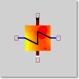
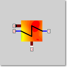
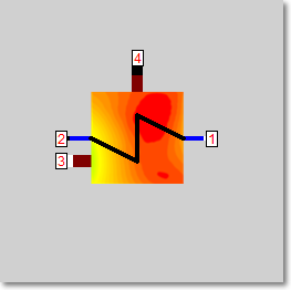
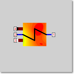
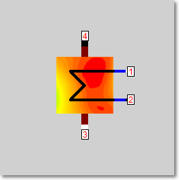
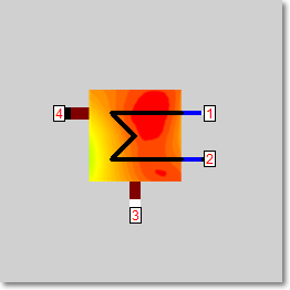
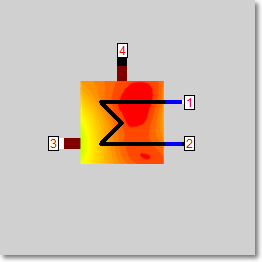
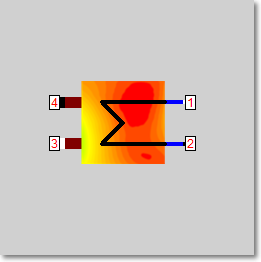
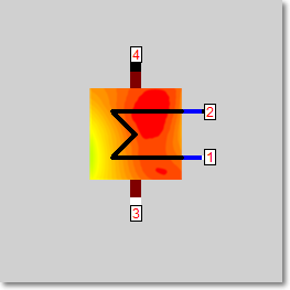
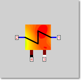
Line connections |
|
|
|
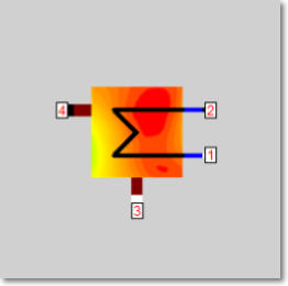
1 |
Fluid inlet primary |
|
|
2 |
Fluid outlet primary |
|
|
3 |
Fluid inlet secondary |
|
|
4 |
Fluid outlet secondary |
|
General User Input Values Results Characteristic Lines Physics Used Displays Examples
Component 126 is mainly based on Component 119 (Indirect storage). The expansion consists in the fact that a second fluid (secondary side) is introduced into the calculation mesh. It is in thermal contact with the storage and thus also with fluid 1 (primary side). The influence of the flow type and the geometry of the real structure on the heat transmission are considered by the heat transfer coefficients. They are specified for the transfer surfaces between the walls and the outside wall of the fluid. The basic pattern thus follows the concept of a double-pipe heat exchanger with respect to following scheme:
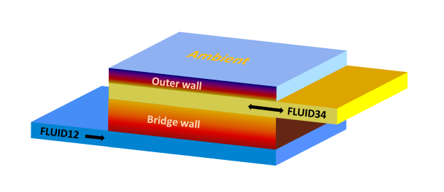 |
A modeling equivalent to the pipe has the advantage that a large number of technical applications can be related to the theory of heat transfer in pipes. Another advantage of the pipe geometry is the cycle-symmetric temperature distribution and heat transfer, so that the calculation of the temperature field is reduced to one radial component over the profiles (y-axis of the calculation mesh) and one along the direction of flow (x-axis of the calculation mesh).
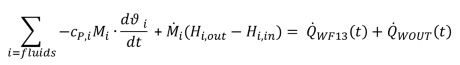
The transient heat conduction in the separation wall between the fluids as well as in the outer boundary wall becomes numerical, calculated with the Crank-Nicolson algorithm analogously to Component 119. The overall balance equation gets in comparison to steady state heat exchangers an extension in terms of sinks and sources as shown in next formula:
 |
Please see also chapter 2.2 in "Physics Used".
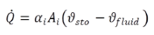
For t -> infinite, the exchanged amounts of heat will reach the values of the steady state case, what means that the 3 characteristic equations used for calculating heat transfer a valid again::
This system of equations is going to be solved during all calculations in order to get the steady state solution asMacro (partial mode) --> Insert... a long term asymptote. This means always accordance to other steady state results.
This transient module is in equivalence to component 119 also controlled by the time series dialogue.
There are three macros (partial models), which demonstrate the usage of this component. You can insert them in your model by clicking on the menu entry "Insert --> Macro (partial mode) --> Insert...". Then select one of the entries "Transient heating surface", "Transient heating surface shape 2" or "Transient heating surface shape 3". After inserting the macro into your model, open the macro to inspect its data. In order to be able to calculate with this, boundary values (component 1) must be connected to the open line inputs and a time series must be created.
|
FMODE |
Flag for calculation mode Design/Off-design =0: Global=1: local off-design (i.e. always off-design mode, even when a design calculation has been done globally) =2: special local off-design (Special case for compatibility with the earlier Ebsilon-versions, should not be used in new models, because the results of the real off-design calculations are not always consistent) = -1: local design (i.e. always design mode, even when a off-design calculation has been done globally) |
|
FINIT |
Flag: Initializing state =0: GLOBAL controlled by variable "Transient mode" in Model Options |
|
FINST |
Flag: Transient calculation mode =0: Transient solution according to time series table |
|
FFU |
Flag: On-/off-switch =0: Heat exchanger off (Only calculation of pressure drops) |
| AWF13 |
Heat transfer area of separation (bridge) wall |
| FVOL |
Flag: Part-load pressure drop, consideration of mass and or volume =0: without influence of volume DP/DPN = (M/MN)**2 |
| FDPNUM |
Pressure loss handling in the numerical solution =0: Using the average fluid pressure between inlet and outlet |
| FDP12RN |
Flag for the type of definition of the primary pressure loss =1: absolute (DP12N=DP12RN) |
| DP12RN |
Pressure loss 12 (nominal) [absolute or relative to P1] |
| FDP34RN |
Flag for the type of definition of the primary pressure loss =1: absolute |
| DP34RN |
Pressure loss 34 (nominal) [absolute or relative to P3] |
|
FALPH12
|
Flag: Determination of the heat transfer coefficient alpha for primary fluid to separation wall =0: always constant value AL12N |
| AL12N |
Heat transfer coefficient alpha for primary fluid to separation wall (nominal, only visible if FALPH12 = 0|1) )
|
| EX12 |
Exponent for heat transfer coefficient to calculate AL12 |
| EALPH12 |
Function for calculation of AL12, equals return value of evalexpr (type real) |
| FALPH34 |
Flag: Determination of the heat transfer coefficient alpha for secondary fluid to separation wall =0: always constant value AL34N |
|
AL34N
|
Heat transfer coefficient alpha for secondary fluid to separation wall (nominal, only visible if FALPH34 = 0|1) )
|
| EX34 |
Exponent for heat transfer coefficient to calculate AL34 |
| EALPH34 |
Function for calculation of AL12, equals return value of evalexpr (type real) |
| DAL34DT | Additional partial load gradient for AL34 - see component 61 The temperature dependency of AL34 can thus be influenced - default value up to release 16: 0.0005 |
|
FALPHO
|
Flag: Determination of alpha outside =0: From constant value ALPHO |
| ALPHO |
Outer heat transfer coefficient (to ambient) |
| EALPHO |
Function for calculation of ALPHO, equals return value of evalexpr (type real) |
| THISO |
Thickness of insulation |
| LAMISO |
Heat conductivity of insulation |
| FALGINST |
Flag: Switch for transient calculation modes =1: Crank-Nicolson-Algorithm |
| FFLOW |
Flag: flow direction =0: Counter Current |
| TAUADBW |
Correction factor for time constant of the bridge wall (reduced physical model only) |
| TAUADOW | Correction factor for time constant of the outer wall (reduced physical model only) |
| LAMADJ |
Multiplication factor to 1/LAMBDA - the walls heat conductivity resistance (reduced physical model only) Setting LAMADJ=0 is equivalent to neglecting the walls heat conductivity resistance: either the wall thickness is infinitely small or lambda value is infinitely high Setting LAMADJ=1 is equivalent to computing the walls heat conductivity with the original value of LAMBDA and wall thickness LAMADJ<1 leads to decreasing the walls heat conductivity resistance LAMADJ>1 leads to increasing the walls heat conductivity resistance |
|
FADAPT |
Flag: Switch for using adaption polynomial ADAPT / adaptation function EADAPT = 0: Not used and not evaluated |
|
EADAPT |
Input of Adaptation-Function |
|
TOLXECO |
Tolerance for evaporation in an economizer. If the steam content X at the economizer outlet is > TOLXECO, a warning message is issued. If it is > 2*TOLXECO, an error message is issued. |
|
PINPMIN |
Minimum value for the pinch point (KA is reduced automatically if the pinch point would fall below this value) |
| LSTO12 | Length of primary flow FLUID12 |
| LSTO34 | Length of secondary flow FLUID34 |
|
AWOUT |
Heat exchanging area of outer wall |
| MWF13 |
Mass of separation wall between fluids (bridge wall) |
| MWOUT |
Mass of outer wall |
|
FVFLUID |
Flag: Switch for calculation of fluid volumes =0: Given from specifications VFLUID12, VFLUID34 |
|
VFLUID12 |
Volume of primary FLUID12 |
|
VFLUID34 |
Volume of secondary FLUID34 |
|
FDATABW |
Flag: Property data source and interpolation =1: Constant from specification values RHOBW, LAMBW und CPBW
=3: From characteristic lines <CRHOBW, CLAMBW, CCPBW |
|
RHOBW |
Density of bridge wall at TREFBW |
|
DRHOBW |
Density change per degree of separation wall |
|
LAMBW |
Heat conductivity of bridge wall at TREFBW |
|
DLAMBW |
Heat conductivity change per degree of bridge wall |
|
CPBW |
Specific heat capacity of bridge wall at TREFBW |
|
DCPBW |
Specific heat capacity change per degree of bridge wall |
|
TREFBW |
Reference temperature for RHOBW, LAMBW, CPBW of separation wall (relevant for FDATABW = 2) |
|
FDATAOW |
Flag: Property data source and interpolation =1: Constant from specification values RHOOW, LAMOW und CPOW
=3: From characteristic lines CRHOOW, CLAMOW, CCPOW |
|
RHOOW |
Density of outer wall at TREFOW |
|
DRHOOW |
Density change per degree of outer wall |
|
LAMOW |
Heat conductivity of outer wall at TREFOW |
|
DLAMOW |
Heat conductivity change per degree of outer wall |
|
CPOW |
Specific heat capacity of outer wall at TREFOW |
|
DCPOW |
Specific heat capacity change per degree of outer wall |
|
TREFOW |
Reference temperature for RHOOW, LAMOW, CPOW of outer wall (relevant for FDATAOW = 2) |
|
FSPECM |
Flag: Handling of system mass of FLUID12 and FLUID34 =1: System mass neglectible |
|
FTTI |
Flag: Handling of temperature during time interval 1: Average temperature for time step interval |
|
FTSTEPS |
Flag: Specification of (sub-) time steps =1: By specification value TISPEP |
|
ISUBMAX |
Maximum number of time sub steps for initialization |
|
IERRMAX |
valign="top" width="558">
Maximum allowed error for initializing step |
|
TISTEP |
Time step, always valid while transient calculation |
|
NFLOW |
Number of points in flow-direction (max. 100) |
|
NRADBW |
Number of radial points in y-direction in bridge wall, (between Fluids, max. 30) |
|
NRADOW |
Number of radial points in y-direction in outer wall, (max. 30) |
|
FFREQ |
Flag: Frequency of transient calculations =1: At each iteration step |
|
TMIN |
Minimum value of wall temperatures |
|
TMAX |
Maximal value of wall temperatures |
|
FSTAMB |
Flag: Definition of ambient temperature =0: Definition specification value (TAMB) |
|
TAMB |
Ambient temperature |
|
ISUN |
Index for solar parameter |
|
TIMETOT0 |
Total time at start of calculation |
|
FRELDIA |
=0: heat exchanging area bridge wall AWF13 relates to inner diameter of tube DI =1: heat exchanging area bridge wall AWF13 relates to outer diameter of tube DA |
|
QN |
Heat exchanger efficiency (nominal) =Q34 |
|
M1N |
Primary mass flow(nominal) |
|
M3N |
Secondary mass flow(nominal) |
|
V1N |
Specific volume for primary inlet (nominal) |
|
V3N |
Specific volume for secondary inlet (nominal |
|
P1N |
Pressure for primary inlet (nominal) |
|
P3N |
Pressure for secondary inlet (nominal) |
|
TM34N |
Mean flue gas temperature (nominal) TM34N=(T3N+T4N)/2 |
The parameters marked in blue are reference quantities for the off-design mode. The actual off-design values refer to these quantities in the equations used.
Generally, all inputs that are visible are required. But, often default values are provided.
For more information on colour of the input fields and their descriptions see Edit Component\Specification values
For more information on design vs. off-design and nominal values see General\Accept Nominal values.
|
Q21 |
Transferred heat to primary flow FLUD12 (in steady state cases =QT and Q34, during transient calculations heat flow from separation wall to fluid) |
|
QT |
Transferred heat through walls (Please note: while doing transient calculations this result doesn´t make sense anymore) |
|
Q34 |
Transferred heat from secondary FLUD34 (in steady state cases =QT and Q12, during transient calculations heat flow to the walls) |
|
KA |
Overall heat transfer coefficient times area from steady state calculation |
|
DTM |
Logarithmic mean temperature difference from steady state calculation |
|
DTLO |
Lower terminal temperature difference |
|
DTUP |
Upper terminal temperature difference |
|
REFF |
Calculated effectiveness (=actual heat transfer/theoretical maximum in case of infinite size) |
|
X2 |
Steam content (X) at primary outlet |
|
AL12 |
Calculated heat transfer coefficient FLUID12 to separation wall |
|
AL34 |
Calculated heat transfer coefficient FLUID34 to outer and separation wall |
|
DP12 |
Pressure loss primary |
|
DPREF12 |
Nominal pressure loss primary |
|
DP34 |
Pressure loss secondary |
|
DPREF34 |
Nominal pressure loss secondary |
|
VM1 |
Specific volume of FLUID12 at inlet conditions (nominal) |
|
VM3 |
Specific volume of FLUID34 at inlet conditions (nominal) |
|
RADAPT |
Result ADAPT / EADAPT |
|
M1M1N |
Related primary mass flow |
|
M3M3N |
Related secondary mass flow |
|
KAKAN |
Related kA-value |
|
KAN0 |
KAN due to KA value |
|
TAVBREND |
Mean caloric temperature of the separation wall at the end of the time step |
|
TAVWOEND |
Mean caloric temperature of the outer wall at the end of the time step |
|
T2AV |
Mean outlet temperature of FLUID12 |
|
T4AV |
Mean outlet temperature of FLUID34 |
|
TX2BEG |
Temperature T2 in the beginning of the time step |
|
TX2END |
Temperature T2 at the end of the time step |
|
TX4BEG |
Temperature T4 in the beginning of the time step |
|
TX4END |
Temperature T4 at the end of the time step |
|
QSTO |
Heat stored in all walls during time step |
|
QAV12 |
Mean heat flow from separation wall to FLUID12 |
|
QAV34 |
Mean heat flow from FLUID34 to all other walls |
|
QAVLOSS |
Mean heat flow from outer wall to ambient |
|
QENDO |
Heat flow from walls to ambient at the end of time step |
|
RALPHO |
Heat transfer coefficient to ambient |
|
THBRW |
Equivalent thickness of separation wall |
|
THOW |
Equivalent thickness of outer wall |
|
REDIA12 |
Equivalent diameter primary FLUID12 |
|
REDIA34 |
Equivalent diameter secondary FLUID34 |
|
MFL12 |
Mass of FLUIDS12 in primary ducts |
|
MFL34 |
Mass of FLUIDS34 in secondary ducts |
|
RELQQ |
Relaxation theoretical/numerical heat flow |
|
TIMEINT |
Total time of the actual time step |
|
TIMETOT |
Total time of the simulation |
|
TIMESUB |
Integration time of the sub steps |
|
INSFRAC |
Fraction of transient calculation steps |
|
ISUB |
Number of sub time steps |
|
TISUBREC |
Recommended time step |
|
PREC |
Precision indicator |
In order to set up temperature dependent material properties, three characteristic lines are introduced. All plots showing the temperature on their X-axes:
All other "characteristic lines" form a circular buffer. The user doesn´t have to take care of them.
Corresponding to this "characteristic lines", there are also result arrays.
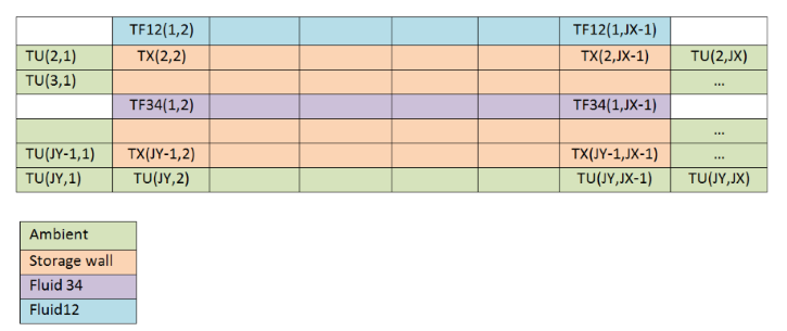
Specification matrix MXTSTO and result matrix RXTSTO
The matrix MXTSTO is linked to the result matrix RXTSTO in the same way as the characteristic curves and result arrays mentioned above.
The distribution of the values in the storage and the fluids is stored in both matrices (default matrix MXTSTO for time step t-1 and result matrix RXTSTO for time step t).
For the structure of the matrices, see matrices of component 126.
|
|
In order to handle complex structures of heat exchangers, the storage or pipe masses MWF13 (separation/bridge wall between the two fluids), MWOUT (outer wall of the device), the exchanging area of the separation wall AWF13 and the outer wall AWOUT can be set by the user as well as the length of flow for both of the fluids stored in the variables LSTO12 and LSTO34.
These parameters give a geometric equivalent to wall thickness derived from the geometry of pipes.
Case FRELDIA = 0 (AWF13 related to inner diameter of tube DI)
DI13 = AWF13 / (LSTO12*p) and DIWOUT = AWOUT / (LSTO34*p)
The corresponding "outer diameter" DA can be specified accordingly :
|
|
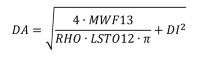
Case FRELDIA = 1 (AWF13 related to outer diameter of tube DA)
DA = AWF13 / (LSTO12*p)
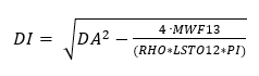
The corresponding "inner diameter" DI can be specified accordingly :
|
|
Hence this leads to wall thickness using the correlation s = 0.5 * (DA-DI).
In dependency on the switch FVFLUID the volume of the duct can be chosen freely with no respect to the other geometric parameters. On the other hand, it is possible to force a calculation using the pipe geometry.
For a certain conductivity of temperature
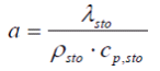 (2.1) (2.1) |
and given distances dXnbsp;and dY to the neighbour points, the distribution of temperatures Θ in the walls is calculated by solving the differential equation for all discrete elements in the storage.
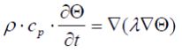 (2.2) (2.2) |
simplified to two dimensions the yield is:
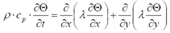 (2.3) (2.3) |
Changes to the temperatures starting at an initial state always occur due to heat flow through the walls and the insulating surface (see also chapter 3).
Tip: In order to carry out certain calculations it can be necessary to ignore the outer wall by setting area and mass nearly to zero, while giving a y-resolution only of one element. Insulation can also switched off with suitable values for THISO and LAMISO.
There are 2 algorithms in component 126 for the computation of the wall temperature. Like in comp. 119 for FALGINST=1 the equation (2.3) is solved numerically using Crank-Nicolson-Algorithm . For FALGINST=4 the combined analytic and numeric method is used instead.
Heat flow between the walls and the fluids depends on position and time, what is described mathematically by linking the convective 2.4 to the conductive terms 2.5:
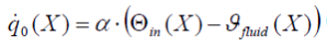 (2.4) (2.4) |
and
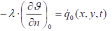 (2.5) (2.5) |
whereas  represents the temperature of the wall area facing the fluid.
  is the temperature of the media and
  indicates that the direction of the heat flow is orthogonal to the flow direction of the fluid. Heat flow at outer wall will be calculated equivalently.
Heat fluxes at the walls induce a change of the media temperatures, which also influences the whole 1-D grid of the fluid. Gradients orthogonal to the flow direction and the flow dynamics as well will be neglected in order to keep the model simple and save CPU-time. Calculation of time dependent changes of the temperature profile will be done based on mass and energy balances for every volume element.
 (2.6) (2.6) |
and
 (2.7) (2.7) |
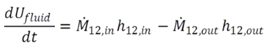
The internal energy of a fluid element is given by 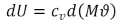 , introduced to eqn 2.7 the result is:
 (2.8) (2.8) |
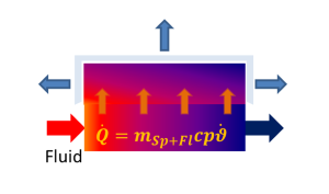
Left side of this equation shows the energy stored in the fluids, while the right side gives the resulting energy flows from the walls trough the boundaries. Summing up those terms and the thermal losses gives the change of the internal energy of the walls of the heat exchanger.
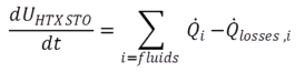 (2.9) (2.9) |
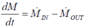
Mass of a fluid element is defined by:
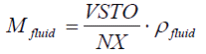 (2.10) (2.10) |
All property calculations of the media are based on the EBSILON media library.
FSPECMXX=1: In case of continuous flow Min = Mout conditions and neglectible fluid mass in comparison to the mass of the wall(s), left side of eqn 2.8 is set to zero, what simplifies the following calculation to:
 (2.11) (2.11) |
FSPECMXX=2: In case of continuous flow Min = Mout or a zero mass flow Mfluid = 0, there´s no change of the masses in the duct pipe. But if the second condition concerning the mass ratio and coupled to this the energy content of the fluid has to be taken into account, it´s necessary to change eqn 2.8 to the following:
 (2.12) (2.12) |
Example: Cooling down a stagnant thermo liquid in duct.
FSPECMXX=3: Fluid mass inside the pipe is variable, what can be the result of changing density as a function of pressure and temperature. In assumption of a constant duct volume different mass flows at inlet and outlet can occur.
Example: Evaporation from a vessel after a pressure drop or temperature jump on the secondary side
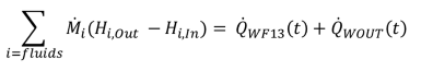
The calculation of the heat fluxes is done using eqn 2.8 combined with the settings given by switch FSPEM. In case of neglectible fluid mass the energy balance for both of the fluids appears as following:
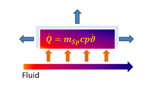 |
The mass of the storage, whose changes of temperature induces a heat flow (Q0(t)), only consists of the wall elements. The fluids are connected thermally via the following equation:
 (2.13) (2.13) |
In the same way the calculation of heat losses to the ambient (blue arrows) is carried out and passed to the result values of QAVLOSS and QENDO. The transient storage behaviour is realized by solving the volume integral of all temperature changes:
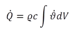 (2.14) (2.14) |
Balancing all heat flows (according to eqn 2.13) delivers the stored amount of thermal energy with further integration concerning the time step. The result is passed to the variable QSTO:
The balancing of all heat flows (according to Eq.(1)) provides the stored heat quantity with a further integration over the time step, stored in the result variable QSTO:
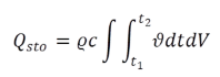 (2.15) (2.15) |
This value QSTO divided by the interval of the time step Dt shows the mean heat flow QAV12 between separation wall and FLUID12 and also that between separation wall, outer wall and FLUID34 set to result variable QAV34.
Tip: Depended on the magnitude of the temperature gradients and the choice of the time step, it is not possible to get a closed energy balance. If greater miss balances appear, it will be reasonable to reduce the time interval or do a refinement of the time step by adjusting FTSTEPS.
If simulations are done with respect to the fluid mass (FSPECMXX = 2,3), balancing becomes different as shown below:
 |
Left side of eqn 2.8 is not zero anymore, hence fluid mass is considered in this equation. The walls and fluids as well are acting as transient energy storage.
The switch FINST generally controls the transient behaviour of the component.
FINST=0: Intervals of the time depended calculation steps are given by the time series dialogue, which takes control of the whole calculation. All transient terms including thermal storages in the equations are going to be solved.
FINST=1: The calculation of the component is steady state, e.g. such a kind of heat exchanger is going to be simulated. Any changes of specifications concerning the heat transfer will result to a new steady state solution for the component. All transient parts of the equations are not considered.
Initializing the simulation using the switch FINIT
FINIT=1: Due to the specifications the heat exchanger is going to be initialized in steady state. In fact that means, a first transient calculation is carried out to lead the system in the state of the long term asymptote. This will be stored to all matrices containing the distribution of temperatures as an initial guess for the following simulations.
Please note:
Specifying the coefficients AL12N and AL34N fixes the overall heat transfer coefficient k shown in eqn 3.1. With all terms forming k are known, the calculation as quite trivial, but other way round it is not possible to get the parts of the sum out of a certain value of k!
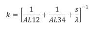 (3.1) (3.1) |
In case of this component the heat exchanging area (AWF13) has also to be specified to make the transient calculation work. As a consequence of this, the value kA is fixed, so the steady state and transient part of the simulation get the same input, what is necessary to ensure consistency. Hence design cases which calculate a certain value of kA are not reasonable and therefore this option is not given here.
FINIT=2: Calculations are carried out according to the specifications of the time series dialogue. Results of the previous step generate the input to the next.
 |
Form 1 |
 |
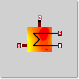
Form 2 |
 |
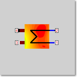
Form 3 |
 |
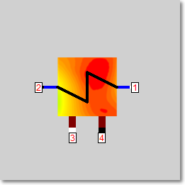
Form 4 |
 |
Form 5 |
 |
Form 6 |
 |
Form 7 |
 |
Form 8 |
 |
Form 9 |
 |
Form 10 |
 |
Form 11 |
 |
Form 12 |
 |
Form 13 |
 |
Form 14 |
Click here >> Component 126 Demo 1 << to load example 1 (Economizer with characteristic lines for material properties).
Click here >> Component 126 Demo 2 << to load example 2 (General heat exchanger with losses to ambient).
Click here >> Component 126 Demo 3 << to load example 3 (Super Heater with evaporation).
 (1)
(1) (1)
(1)