
Technically, a power plant comprises of components, which are connected with one another by means of pipes. The transfer of energy takes place through the so-called fluids (water, steam, flue gas, air etc.), whose state equations are present in the form of standardized polynomials.
An exact thermo-hydraulic modeling of the respective load points of the real power plant would permit to indicate the errors in the available measurement values. The stationary simulation programs available today, which so far have been used for planning and design calculations, enable a high modeling accuracy in view of the mass flow and energy balancing, whereby specific parameters in the physical component equations are described by characteristic lines or curves, which depict the real behaviour quite exactly. In view of the data validation as per the guideline VDI 2048, along with their uncertainties, the ones present in the equations used (e.g. the steam cone law) and in the data must also be taken into account.
If the measurement values are expected to be detected in percentages, then the accuracy of the computing model should correspond to this, as otherwise the difference in the measured value and the calculated value could be caused by inaccuracies in the modeling. Therefore, before the data validation can be done properly, the suitability of the computing model and of the intended evaluations must be demonstrated. Thereby, the requirements of the criteria catalogue of the VDI for the certification must be fulfilled and the system of the auxiliary conditions must be x-rayed for any possible discrepancies or inaccuracies. The auxiliary conditions are derived automatically from the model topology created with the EBSILON®Professional user interface and from the component specifications. The generated balancing equations can be formally viewed as correct, because EBSILON®Professional is working error-free for years in this area. However, it must be noted that discrepancies in the modeling lead to contradictions (e.g. ignoring the leakage flows). Hence, the balancing violations must be checked with the raw data (see error analysis).
The equations used for the individual components can be called and displayed from the system help by a mouse click. This will be explained by taking the example of the help text of a steam turbine (Component 6). With the simplification that the mechanical efficiency is ETAMN=1 and the inlet and outlet loses are DH1LN=DH2LN=0, the given calculations can be summarized as follows:
(1) P1 = SQRT (P2^2 + ((M1/M1N)^2)*(V1/V1N)*(P1N^2-P2N^2) ) (Steam cone law according to Stodola) See also: Part-load - Steam Turbine
(2) P3 = P2
(3) P4 = P2
(4) H2 = H1 - (H1 - H2S) * ETAI , where H2S results from P2 and S1 from the water-steam table
(5) H3 = H2
(6) H4 = H2
(7) Q6 = Q5 + M1 * (H1 - H2) (energy balance, losses ignored)
(8) M2 = M1 - M3 - M4 (mass flow balance, losses ignored)
Mi, Pi, Hi, Vi, Si, Qi respectively are the mass flow, pressure, specific enthalpy, specific volume, entropy and power at the connection i of the component (as shown in the figure below, according to the connection naming in EBSILON®Professional). For simplicity, the losses in the mass flow and energy balances are ignored, which must be taken into account when modeling a real plant (e.g. branching at the outlets 2, 3 or 4).
Since the steam-cone law does not apply strongly, it can also be taken from the auxiliary conditions by setting the flag FP1N to "P1 specified from outside" in case of turbines. The measured value is then used as default value in the extraction. If such a value is not present, then a pseudo measured value can be created, whose value is taken from the simulation calculation with Stodola. The related confidence interval is to be set according to the assumed uncertainty. In case of a noteworthy change of flow in the validation, an iterative handling of the pressure default can become necessary, which can be done through simulation calculations with validated values. Thereby, the expansion course over the entire turbine stage (see h,s-diagram) must be taken into account.
To get an overview of the equations used, (display of the auxiliary conditions in balance form), one can activate the Equations list.
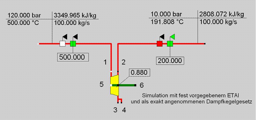
However, specification data is contained in the component equations, which can be inapplicable. This is shown by the following simulation example:

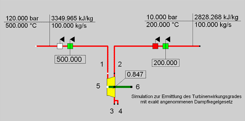
The equations were generated correctly, but the deviation of the calculated outlet temperature (191.8 °C) from its measured value (200 °C) indicates an invalid specification of the isentropic efficiency (ETAI). In this way, inaccuracies can be detected by doing a simulation with the raw data. All the uncertainties must then be included in a validation calculation i.e. quantities such as ETAI and losses must also be validated. However, here only the advantages of the preceding simulation will be discussed.
In the example, the component can derive in the identification mode the applicable ETAI value from the outlet temperature measurement:

If the outlet temperature has been measured wrongly, then it is expressed in the results of the subsequent component. The simulation results for the entire model thus provide a valuable help for checking the measured values and the model.
If around a component a measured value deviates very strongly from the calculated value, then along with a faulty measuring, the following could also be a reason: false parameter setting of the component, invalid selection of the component or violation of the equations used (auxiliary conditions), which might have been caused by a damage to the component.
This will be explained by taking the example of the steam cone law. For calculating the pressure in a steam turbine disc, the steam cone law is selected via the specification screen in the following form:
p1^2 = p2^2 + ((m1/m1n)^2)*(v1/v1n)*(p1n^2-p2n^2) (the meaning of the symbols can be taken from the component help)
The equation is completely valid at nominal load at the design point, while the accuracy decreases in the off-design mode. All quantities of the equation and the equation itself must be viewed as free of errors. While p1, m1, v1 go directly in the balancing equation with their uncertainties, this is not given for the nominal values, the more so as these are not fixed, but dependent on off-design i.e. the true nominal values actually do not exist. Under consideration of the nominal quantities and the formula itself, a suitable confidence interval is set for the calculated value p2 and for p2 the value calculated in the simulation with the steam cone law is entered as estimated value in a pseudo measurement value. The steam cone law is then deactivated in the validation and the pseudo measurement value is specified as the default capable of being validated. If there is a very big difference between the calculated p2 and an eventually measured extraction pressure, then either this pressure loss must be modelled, in a way that it can be validated, for the estimated pressure loss on the way to the measurement point (the condensate saturation temperature must be matching at the related preheater), or the nominal values of the turbine must be modified. If the nominal pressure values are modified, then it must be noted that the turbine efficiency (can be validated) takes up values not permitted, which would lead to another contradiction in the super-heated steam range for a reliable measurement of the outlet temperature (can be validated). Setting the parameters of the power plant model requires special care, as shown by this example. Naturally, the observations are simpler for the mass flow and energy balances. If necessary, deviations can be modelled here in a way, such that these can be validated, with simple means (e.g. for heat loss at a component assumed to have an adiabatic flow).
The computing model can be checked on one hand by comparing it with the precise design calculations of the supplier for the components and for the entire plant, and on the other hand, by carrying out corrected acceptance and precision measurements at the components. The adaptation of the specification parameters and the characteristic lines should finally lead to the necessary accuracy.
If this aim is reached, the data validation can be started. To solve the equation system of the model, the specification of a few measurement values that define the cycle (pressures, temperatures, mass flows) is sufficient. The calculation produces the thermodynamic process model, comprising of component and pipe data. Owing to the defectiveness, it is best to let all the measurement values flow in the evaluation. This results in an over-determined equation system, which can be traced back to a specific error with the method of the smallest mean square error, whose symmetric matrix results in validated measurement values in a simple resolution. The maintenance of the mass flow and the energy balances for the components and the entire plant must thereby the considered as auxiliary condition in the adaptation calculation. The process image validated at the model represents the most probable process state i.e. the differences between the measurement values and the related validated values specify the probable error (with the sign) of the measurement values.