EBSILON®Professional Online Documentation


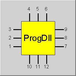
The number of pins has been expanded to 10 inlets and 10 outlets. It is up to the programmer of the DLL, how these are to be used.
|
Line connections |
|
|
|
1 |
Inlet 1 |
|
|
2 |
Inlet 2 |
|
|
3 |
Inlet 3 |
|
|
4 |
Inlet 4 |
|
|
5 |
Inlet 5 |
|
|
6 |
Inlet 6 |
|
|
7 |
Outlet 1 |
|
|
8 |
Outlet 2 |
|
|
9 |
Outlet 3 |
|
|
10 |
Outlet 4 |
|
|
11 |
Outlet 5 |
|
|
12 |
Outlet 6 |
|
|
13 |
Outlet 7 |
|
|
14 |
Outlet 8 |
|
|
15 |
Outlet 9 |
|
|
16 |
Outlet 10 |
|
|
17 |
Inlet 7 |
|
|
18 |
Inlet 8 |
|
|
19 |
Inlet 9 |
|
|
20 |
Inlet 10 |
|
The component 65 can be used to link a self-written program for calculating a component in Ebsilon. The linking is done in the form of a DLL. Suitable development tools must be available for creating such a DLL.
When the DLL is called, the data concerning the corresponding component are transferred to this DLL from the Ebsilon model, which can then carry out specific calculations with this data. The result values are imported by Ebsilon.
With this component it is possible, like in the case of component 93 (KernelScripting), to trigger equations. For this the use of the “extended interface” and programming in C++ are required.
The path to the DLL can be specified directly at the component. Before, this was only possible in the general settings, comprehensively for all models and components. This way, the use of different DLLs in one model has become possible.
The "Ports" tab window shows the fluid types assigned to the component connectors.
There is an entry for each connector. It includes the connectors number and a combo box, which always displays the fluid type currently assigned.
You can change the fluid type of the connection points by clicking in the combo box fluids-type and selecting a type from the list displayed.
It is possible to fade out an connection completely by specification of "None" as fluid.
Note:
There are characteristic lines, result arrays, specification matrices, and result matrices for these components, too. It is possible to have result values calculated in each
iteration step. See tab "Calculation" -> "Calculation options" -> "Result calculation" -> (1) "Calculate results at each iteration step"
There are additional interfaces for Component 65. See tab "Experts" and notes in chapter "Editing components" -> tab "Experts".
|
DLLPATH |
Alternative path to the Programmable-Dll This entry is optional. If no path is specified here, the path is taken from the general options. |
|
FSEQ |
Position in calling sequence Like in Parent Profile (Sub Profile option only) Expression =0: Parallel to other components =1: Late, after fluids are recalculated |
|
FTAKEOVERNOMINALVALUES |
Take over nominal values : After a successful (local) partial power calculation, it is decided on the basis of this specific value whether the values from SPEC1, ..., SPEC80 are adopted as nominal values.
Like in Parent Profile (Sub Profile option only) Expression = 0: call function XUI_hasNominalValues and proceed based on the result
|
|
FPROG |
Program-ID (Classification of the sub-type of the component specified by the user) |
|
SPEC1,..., SPEC80 |
Specification values defined by the user (can also be used as nominal values) |
Generally, all inputs that are visible are required. But, often default values are provided.
For more information on colour of the input fields and their descriptions see Edit Component\Specification values
For more information on design vs. off-design and nominal values see General\Accept Nominal values
You will need your own C-compiler for creating a program in C, which generates a dynamic link library (DLL) that replaces the DLL Programmable.dll. This DLL is shipped together with EBSILON®Professional (compiled and linked with Visual C++ 6.0 ).
Several types of self-defined components can be implemented, which can then be differentiated by means of the specification value FPROG. This value defines the type to be used. Since the Programmable.DLL is available only once, each type can be used in models or cycles.
The Programmable.dll is used by the calculation kernel of Ebsilon and not by the graphical user interface (EbsOpen, for instance, can be used for exchanging data with the GUI). During the solution procedure, it is activated in each iteration step and is therefore part of the iteration process. Therefore it is important for the DLL to possess corresponding convergence properties. Otherwise the calculation will need more iteration steps or will not converge any more at all.
The calculation kernel activates the DLL with an interface described in the header files EbsUser.h and xui.h. These files can be found in the directory Examples\xui_dll.
The DLL interface for C consists of a single function with the name EbsUser_Comp65. As return value, this function yields an integer that can be specified at will. The calculation kernel interprets this return value as follows:
The DLL interface for C++ consists of several functions whose names all begin with “XUI_“. The description of these functions is contained in the header files EbsUser.h and xui.h (only available in English).
In case of error or warning, your return value will be displayed in the error analysis:

The only argument of the function EbsUser_Comp65 is a pointer to a EBSPROG_CALC_DATA structure. This structure is defined as
typedef struct {
int compno; // Component number (1 = first comp.65 in your drawing; 2 = 2nd comp.65 ...)
int nrule; // number of rule to calculate (= first specification value)
int nspecs; // number of specification values
int nresults; // Number of result values
int n_inlines; // number of input lines
int n_outlines; // number of output lines
int n_materials; // maximum number of materials in the composition of a line
EBSPROG_PARAMS calcparams; // Calculation parameters
double *specs; // Array of 'nspecs' component specification values
// Blank values are indicated as '-999'
double *results; // Array of 'nresults' component result values
EBSPROG_LINEVAL *in; // Array of 'n_inlines' input line values
EBSPROG_LINEVAL *out; // Array of 'n_outlines' output line values
} EBSPROG_CALC_DATA;
Before the Ebsilon calculation kernel calls your DLL, it creates this structure and copies the data from the actual iteration step into this structure. Therefore, in your DLL you have access to all these data in the structure.
Look at the examples in EbsUser.c to see how you can access Ebsilon specification and line values, and specify your results.
The parameter compno indicates the component 65 (there can be several in the cycle), which is currently being calculated.
The parameter nrule is the value that is specified as FPROG in the component property sheet. This may be used to distinguish different types of user-defined components, if you want to implement several ones.
The parameters nspecs, nresults, n_inlines, n_outlines and n_materials indicate the size of the corresponding arrays. You should always use these quantities in your code instead of fixed numbers (like 39, 40, 6) because in future Ebsilon releases the corresponding numbers could change.
EBSPROG_PARAMS is a structure that tells you about the conditions and the settings of the calculation:
typedef struct {
int mode; // Calling mode: Initializing (1), Calculating (2), Finishing (3)
// Mode 1: Receive specification data from Ebsilon and perform your initializing.
// No data transfer back to Ebsilon.
// Mode 2: Receive line data from Ebsilon and perform your calculation.
// Line results are transferred back to Ebsilon.
// Mode 3: Specification values and component results are transferred back to Ebsilon.
int itno; // Number of iteration step (may vary from 1 to 998)
int design; // Design (0) / Off design (1) calculation
int wst; // Water steam table to be used: 0=IFC-67, 1=IAPWS-IF97
} EBSPROG_PARAMS;
The mode parameter can be used by your program if you have to do certain initializing or finishing work, like allocating and deallocating of memory or opening and closing of files.
The parameter itno informs you about the iteration step being executed currently.
The parameter design is important for two reasons:
The wst parameter is needed if you want to call material tables. For consistency reasons, you must use the same formulation of the water/steam tables in your DLL as in Ebsilon.
EBSPROG_LINEVAL is a structure that contains the line values. For the input lines, these values are provided by Ebsilon for your calculation. For the output lines, Ebsilon expects that these values are calculated by your program.
typedef struct {
double p; // pressure [bar]
double h; // enthalpy [kJ/kg]
double m; // mass flow [kg/s]
double ncv; // net calorific value [kJ/kg]
MT_ANALYSE ana; // composition
double fugit; // fugitive portions (coal only)
double rho; // density (oil only)
double zfac; // Z factor (oil only)
int fcoal; // coal type (coal only)
} EBSPROG_LINEVAL;
The MT_ANAYLSE structure is used to specify the material composition. It is defined in material_table.h. See the description of the material table functions for details.
The user must define, how the values of the 6 outlet connections depend upon the input values of the 6 inlet connections.
If you need more than six inlet and six outlet lines, you can combine several of these components (differentiated by the parameter FPROG).
You can call all material-table-functions (water and combustion) from your C program.
You can easily integrate any other programs or APIs available to you by modifying the Make-file and including additional header files.
Note that the calculations you implement are performed in each iteration step of the simulation, and have an influence on the convergence behaviour.
Your document may include several components of type 65. Each must have a valid sub-component number FPROG assigned to it. Each assigned sub-component number (FPROG) must be implemented in your C code or DLL respectively.
Three sample sub-components are given in "Data\Examples\Programmable\ebsuser.c". These examples have been tested with Microsoft Developer Studio 6.0 (Visual C++). The associated documents are stored in the directory data\examples\components\ of the EBSILON®Professional installation directory. Their names are Component_65.ebs, Component_65_2.ebs and Component_65_3.ebs .
Use the file ebsuser.c as shipped with EBSILON®Professional. Before modifying the file, create your own DLL Programmable.dll by compiling and linking this original file.
Do the following: The files
are stored together in the folder Data\Examples\Programmable\, which is selected as the EBSILON®Professionalinstallation directory.
If you have Visual C++ installed, you have to
As a result, ebsuser.obj and the DLL ProgrammableUser.dll will be created.
Replace the Programmable.dll shipped with EBSILON®Professional with the one you have just created by renaming and copying it. Do not forget to backup the original DLL, in case your DLL does not work.
To implement your own sub-component, modify the function EbsUser_Comp65, which is included in ebsuser.c . This function looks like this:
LINKDLL int EbsUser_Comp65 (EBSPROG_CALC_DATA *data)
{
int rc;
switch (data->nrule) {
case 1:
..... code for sub type 1
break;
case 2:
..... code for sub type 2
break;
case 3:
..... code for sub type 3
break;
default:
rc = -999;
break;
}
return rc;
}
Adding a sub component means to add a new case block inside the switch (FPROG).
The available inputs are the fields for
Each parameter includes the values of all six input pipelines.
As examples, the ebsuser.c shipped with EBSILON®Professional includes three sub components (FPROG 1, 2 and 3).
The first example (FPROG = 1) uses all input and all output pipelines. It is the one used in the EBSILON®Professional example Component_65.ebs located in the directory examples\components\ of the installation directory.
The second example (FPROG = 2) (detailed description) uses the input pipelines 5 and 6 and the output pipelines 2 and 3. It is used in the EBSILON®Professional example Component_65_2.ebs located in the directory examples\components\ of the installation directory. The interface to the material tables is used in this example, but only the water table is used.
The third example (FPROG = 3) (Component_65_3.ebs located in the directory examples\components\ of the installation directory) splits up a crude gas mass flow into three mass flows:
The interface to the combustion material tables is used in this example, the net calorific value of the resulting mass flows is calculated.
You can use and modify the make file (Data\Examples\Programmable\Programmable.mak) shipped with EBSILON®Professional. You can use your own compiler, linker, make-file etc. or any other tools you want.
The DLL you create has to be a multithreaded DLL. Do not use MFC.
The available functions are listed below. When the function is called, the input values must be specified as displayed.
The abbreviations used are
|
Abbreviation |
English |
German |
|
Steam |
|
|
|
p |
pressure |
Druck |
|
T |
temperature |
Temperatur |
|
h |
specific enthalpy |
spezifische Enthalpie |
|
s |
specific entropy |
spezifische Entropie |
|
v |
specific volume |
spezifisches Volumen |
|
cp |
isobaric specific heat |
Isobare spezifische Wärmekapazität |
|
x |
quality |
Dampfgehalt |
|
Flue gas |
|
|
|
p |
pressure |
Druck |
|
T |
temperature |
Temperatur |
|
h |
specific enthalpy |
Spezifische Enthalpie |
|
s |
specific entropy |
Spezifische Entropie |
|
v |
specific volume |
Spezifisches Volumen |
|
cp |
isobaric specific heat |
Isobare spezifische Wärmekapazität |
|
x |
water content |
Wassergehalt |
|
xs |
saturation water ratio |
Maximaler Dampfgehalt (gesättigt) |
|
MRAT |
mass ratios |
Massenanteil |
|
VRAT |
volume ratio |
Volumenanteil |
|
MG |
molar weight |
Molgewicht |
|
HU |
lower calorific heating value |
unterer Heizwert |
|
Result► |
Specific enthalpy |
Pressure |
Specific entropy |
Temperature |
Specific volume |
Isobaric specific heat |
Steam content |
|
Input▼ |
|||||||
|
Pressure, temperature |
h = f (p, T) |
|
s = f (p, T) |
|
v = f (p, T) |
|
|
|
Pressure, specific enthalpy |
|
|
s = f (p, h) |
T = f (p, h) |
v = f (p, h) |
cp = f (p, h) |
x = f (p, h) |
|
Pressure, specific entropy |
h = f (p, s) |
|
|
T = f (p, s) |
|
|
|
|
Temperature |
|
p = f (T) |
|
|
|
|
|
|
Specific entropy |
|
p = f (s) |
|
|
|
|
|
|
Specific enthalpy |
|
p = f (h) |
|
|
|
|
|
|
Pressure |
h = f (p) h = f (p) |
|
|
T = f (p) |
|
|
|
Fluids can comprise of various substances. The mass fractions of the individual substances must be specified.
In addition to the input values specified in the tables below, nearly all calculations need these mass ratios too. Only the calculation of the mass ratios themselves needs the volume ratios.
|
Result ► |
Specific enthalpy |
Specific entropy |
Temperature |
Specific volume |
Specific heat |
Fluid water fraction |
Saturation water ratio |
Volume ratios |
Mass ratios |
Net calorific value |
Mole weight |
|
Input ▼ |
|||||||||||
|
Pressure, temperature |
h = f (p, T) |
s = f (p, T) |
|
v = f (p, T) |
cp = f (p, T) |
x = f (p, T) |
xs = f (p, T) |
|
|
|
|
|
Pressure, specific enthalpy |
|
s = f (p, h) |
T = f (p, h) |
|
cp = f (p, h) |
x = f (p, h) |
|
|
|
|
|
|
Pressure, specific entropy |
h = f (p, s) |
|
T = f (p, s) |
|
|
|
|
|
|
|
|
|
only mass ratio |
|
|
|
|
|
|
|
VRAT |
MRAT |
HU |
MG |
|
Result ► |
Specific enthalpy |
Temperature |
Specific heat |
Net calorific value |
|
Input ▼ |
||||
|
Pressure, temperature |
h = f (p, T) |
|
cp = f (p, T) |
|
|
Pressure, specific enthalpy |
|
T = f (p, h) |
cp = f (p, h) |
|
|
only mass ratio |
|
|
|
Hu |
The fuels and the flue gas can consist of several materials. The mass ratios of these materials have to be defined.
In addition to the input values specified in the tables above, nearly all calculations need these mass ratios too. Only the calculation of the mass ratios itself needs the volume ratios.
To define a composition, use only the functions mt_init_analyse () and mt_set_analyse ():
void mt_init_analyse (MT_ANALYSE *analysis,
MT_ANALYSE_TYPE analysis_id);
BOOL mt_set_analyse (MT_ANALYSE *analysis,
MT_ANALYSE_PART component_id,
double portion);
To query a composition, only mt_inq_analyse () must be called:
BOOL mt_inq_analyse (MT_ANALYSE *analysis,
MT_ANALYSE_PART Component_ID,
double *portion);
(the structures are declared in the header file materials_table.h).
The function mt_calc () is available for using the material tables. This function is defined as follows:
BOOL mt_calc (MT_ANALYSE_TYPE table_id, // Type of material (= fluid type) (input)
MT_FUNC_ID func_id, // Requested function (input)
double para_1, // 1st parameter of function (input)
double para_2, // 2nd parameter of function (input, if necessary)
MT_ANALYSE *analyse, // Material composition (input, in case of MT_VRAT_OF_MRAT
// or MT_MRAT_OF_VRAT input and output)
double *result, // Calculated result of the requested function (output)
MT_PHASE_ID *phase_id, // Phase for water (output, if available)
MT_FORMULATION formulation, // Water/steam table formulation to be used (input)
long *error_id); // Error code (0 = success)
All the parameters must be defined. The available data types and the values are defined in the header file materials_table.h.
|
Parameter |
Data Type |
Purpose |
Legal Values |
|
table_id |
MT_TABLE_TYPE |
Specified the material table to be used. |
MT_AT_WATER |
|
func_id |
MT_FUNC_ID |
Specifies the function to be executed. The letters in front of _OF_ specify the result, the letters after the input parameters: e.g. PT means pressure and temperature, thus H_OF_PT means: enthalpy as a function of pressure and temperature |
MT_H_OF_PT |
|
para_1 |
double |
This is the 1st input parameter |
Corresponding to the respective function: |
|
para_2 |
double |
This is the 2nd input parameter |
Corresponding to the respective function: |
|
analyse |
MT_ANALYSE_TYPE |
Specifies the material composition (gas, fluid, coal) . mt_set_analyse to modify or mt_inq_analyse to read the composition. |
The fractions must be entered as double-values. The material type must be: |
|
result |
double |
This is the result value. |
Corresponding to the respective function:: |
|
phase_id |
MT_PHASE_ID |
This results in the phase for water/steam. |
MT_PI_FLUID |
|
formulation |
MT_FORMULATION |
Formulation of the water/steam tables |
MT_FORM_WST67 |
|
error_id |
long |
|
0 in case of success. |
For instance, If you want to calculate the specific enthalpy of steam and you have p and T given, you can specify:
or you want to calculate the specific enthalpy of crude gas and you have p and s given, you can specify:
This example shows the modeling of component 8 (see further below) by using the component 65.
Component No. 8 has three connections:
The following image shows the cycle above modelled by using component 65. Here, the inlets are located at its lower and right side, the outlets at its upper and left side. The specification value FPROG is set to 2.
In contrast to the previous model, now four connectors are used:
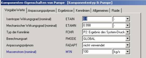
Given below are the specification values of the pump in the original model and the associated code in the file ebsuser.c. The names of the variables are the names used in the Online Help chapter describing component 8 and its equations. The necessary specification values of the pump are specified as constants. The characteristics have not been implemented. This does not matter, because in the original model
case 2:
//
// Case 2 (FPROG = 2):
//
// Modeling a pump as replacement for component 8
//
// For the equations see Online Help of component 8
// The water inlet is connected to input 6 of component 65.
// The pressure to be built up is connected to input 5 of component 65.
// The water outlet is connected to output 2 of component 65.
// The shaft is connected to output 3 of component 65.
//
// The specification values are:
// ETAIN = SPEC1
// ETAM = SPEC2
// M1N = SPEC3
//
// The result values are:
// ETAI = RES1
//
// Note that in C, indexes are starting with 0 (i.e. SPEC1 = specs[0],...)
//
int rc = 0;
double etain, etai; // Nominal and actual isentropic efficiency
double etam; // Mechanical efficiency
double m1n; // Nominal mass flow
double p1,h1,m1;
double p2,h2,m2;
int rcmt; // Return code from mt_calc
double s1,t2s,h2s,dhs,dh,t2,q2,q3;
int ii;
int phase = 0, error = 0; // for water/steam table
MT_FORMULATION form;
// Reading specification values
etain = data->specs[0];
etam = data->specs[1];
m1n = data->specs[2];
// Reading input from water inlet (6) into local variables
p1 = data->in[5].p;
h1 = data->in[5].h;
m1 = data->in[5].m;
// Reading pressure input (line 5) into local variable
p2 = data->in[4].p;
// Calculation of actual efficiency
if (data->calcparams.design == 0) {
etai = etain;
}
else {
etai = etain * (m1 / m1n);
}
// Reading water steam table
form = data->calcparams.wst;
// Equations of component 8
rcmt = mt_calc (MT_AT_WATER, MT_S_OF_PH, p1, h1, NULL, &s1 , &phase, form, &error);
assert (rcmt);
rcmt = mt_calc (MT_AT_WATER, MT_T_OF_PS, p2, s1, NULL, &t2s, &phase, form, &error);
assert (rcmt);
rcmt = mt_calc (MT_AT_WATER, MT_H_OF_PS, p2, s1, NULL, &h2s, &phase, form, &error);
assert (rcmt);
dhs = h2s - h1;
dh = dhs / etai;
h2 = h1 + dh;
rcmt = mt_calc (MT_AT_WATER, MT_T_OF_PH, p2, h2, NULL, &t2 , &phase, form, &error);
assert (rcmt);
m2 = m1;
q2 = m2 * h2;
q3 = (m2 * h2 - m1 * h1) / etam;
// Initialize all output values
for (ii = 0; ii < 6; ii++)
{
data->out[ii].p = 0.0;
data->out[ii].h = 0.0;
data->out[ii].m = 0.0;
}
// Setting the values of the water output
data->out[1].p = p2;
data->out[1].h = h2;
data->out[1].m = m2;
// Setting the values output of the shaft - p and m are necessary dummies
data->out[2].p = 0.01;
data->out[2].h = q3;
data->out[2].m = 1.0;
// Calculation of results in the last iteration step only
if (data->calcparams.mode == 3) {
data->results[0] = etai;
// Determine M1N in design case
if (data->calcparams.design == 0) {
data->specs[2] = m1;
}
}
// Determine M1N in design case in the last iteration step
return rc;
} break;
After the cycle and the code are generated, you can compile and link them for creating the DLL.
Click here >> Component 65 Demo 1 << to load example 1 (simple).
Click here >> Component 65 Demo 2 << to load example 2 (simulation of the pump as shown above).
Click here >> Component 65 Demo 3 << to load example 3 (using analysis).