
EBSILON®Professional Online Documentation


|
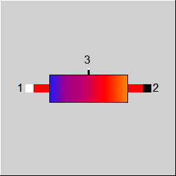
Line connections |
|
|
|
1 |
Inlet |
|
|
2 |
Outlet |
|
|
3 |
Control line, optional (as P) |
|
General User Input Values Physics Used Displays Example
This dynamical component is a variation of the transient separator (component 131). In difference to that component all transfer functions are derived directly from the specified physics and operating parameters. The user doesn´t have to specify time constants or exponents. In certain conditions component 119 can also be substituted. Due to the fact that the solution will be obtained by an analytical function advantages in terms of calculation time will result. All calculation modes of the steady state pipe (component 13) can be used except those which handle electrical resistances. In accordance with all other transient components controlling is carried out using the time series dialog.
While applying a temperature jump to a real pipe via the fluid operation parameters (inlet temperature, mass flow, etc.), a transfer function for the outlet temperature will occur because of the thermal inertia of the pipe walls. All kinds of transients are based on the steady state solution, which is calculated by the specified parameters, e.g. thermal losses by geometry (please see also the remarks on the specification values). In case of changes to the input conditions a "new" steady state will result, which appears not immediately at the pipe outlet, but with a delay caused by the transfer function.
Using compressible flow a transfer function for the fluid mass stored in the pipe can be derived. Combining all the functions is also possible.
By default the design of the pipe will be carried out phenomenically, what means that in design case thermal and pressure losses will be specified. These losses are going to be scaled in part load condition.
Alternatively, it is possible that EBSILON calculates the pressure loss by given geometric parameters.
Another specification will be a given drop of temperature or enthalpy, which is calculated with various part load behaviour. For details please see description of the switch FDN.
Changing the design case simulation between phenomenical and geometrical calculation of pressure loss can be done by the switch FDP.
A third option will be the straightforward specification of the outlet pressure by fixing this value externally in the outgoing line.
In case of a geometrically based calculation of pressure loss it´s required to specify:
• pipe length (LENGTH)
• inner diameter of the pipe (DINNER)
• roughness of the pipe wall (KS)
• possibly a coefficient for an additional pressure drop (ZETA)
At present the transient part of the model is only working properly in case of one phase flow conditions. While calculating the pressure losses geometrically the resulting flow velocity is also displayed. In combination with the specification value VMAX, it is possible to check the allowed maximum of that velocity. Hence a warning will appear when this is out of range.
When using phenomenically based calculation of pressure loss, specification of the design value DP12RN delivers following modes according to the switch FDP12RN :
• absolute pressure drop (=P1-P2) with FDP12RN=1
• relative pressure drop (=(P1-P2)/P1) with FDP12RN=2, 3 or 4
Selections FDP12RN=2,3 or 4 lead to different part load calculations. For details please see description of this switch. The switch FVALDP (FVALDP=1) enables either using a of pseudo measurement point instead of the specification value DP12RN or the use of the control line (connection point 3, FVALDP=2). In this case it´s necessary to connect a stream of logic type to to control the pressure drop by the pressure of the line.
In terms of geometrical and phenomenical calculation, there is another possibility to choose various conditions for the part load calculations. Though geometrical mode is selected, it is possible to activate phenomenical simulation of the part load conditions. This can also be carried out vice versa (geometrical part load coupled to phenomenical design), but seems practically to be meaningless. The switch FVOL takes part in controlling the part load behaviour.
When using an adaption polynom or a kernel expression to adjust pressure drop (FADAPT=-2 or 2), the calculated pressure drop will be multiplied by the result of the polynom or expression.
Implementation of a geodetically induced pressure difference means to specify the value of GH. The calculated pressure difference will be added in all load cases and shown as result.
An off-design pressure loss calculation based on the specific volume at the inlet of the component can lead to higher inaccuracies, if the temperature change between inlet and outlet is high and the flowing medium is compressible / gaseous.
This is why there is the FDPBASE switch, where the mean value of the specific volume between inlet and outlet can also be used and the nominal value V12N (the mean specific volume between inlet and outlet) can be used as a reference value.
All transient components that possess the flag FINIT can be commonly controlled via one global flag.
For this, the flag FINIT has been expanded by the position GLOBAL: 0.
If it is set to this value, the control of the transient simulation will be handed over to the global variable “Transient mode“, which can be found under
Extras \Model Options\Simulation\Transient\ Combo Box "Transient mode".
This will then pass on the desired mode (first iteration or following iteration) to the components. This can be controlled from the time series dialog by means of the expression “@calcoptions.sim.transientmode“.
|
FINIT |
Flag: Initializing state =0: Global, which is controlled via global variable "Transient mode" under Model Options: |
|
FTRANS |
Specification of transfer function: =1: Only transfer function for mass =2: Only transfer function for temperature =3: combined transfer functions |
|
FDN |
Loss types = 1: Heat loss = 2: Temperature loss = 4: Enthalpy loss = 5: Enthalpy loss (wet steam to saturated water) = 6: Relative heat/power loss = -2: T2 given = 3: Temperature loss (superheated steam -> saturated steam){ true for superheated steam, weighted and limited to H2'' - design calculation (full load) T2 = T1-DX - off-design H2 = H1-DQ DQ = M2*T2/(M1N*T2N)*(H1N-H2N) |
|
DN |
Loss (nominal) |
|
FVOL |
Flag for the dependency of the pressure loss on volume =0: without considering the specific volume DP/DPN = (M/MN)**2 =1: with consideration of the specific volume DP/DPN = V/VN*(M/MN)**2 = 2: constant value (load independent): DP = DPN |
|
FDP |
Switch to toggle between phenomenological and geometrical interpretation.
=0: phenomenological specification of the pressure loss in DP12RN |
|
FDP12RN |
Flag for setting DP12RN as absolute or relative value =1: (as previously): DP12RN is used as absolute pressure drop in the design case and as absolute reference pressure drop for off-design calculations: =2: (as previously): DP12RN is used in all load cases as the factor by which the current inlet pressure is multiplied to receive the pressure drop in the design case and =3: DP12RN is only used in the design case as the factor by which the current inlet pressure is multiplied to receive the pressure drop. This pressure is then stored as =4: DP12RN is used in all load cases as the factor by which the current inlet pressure is multiplied to directly receive the pressure drop in the respective load case: |
|
FVALDP |
Validation of the pressure drop =0: DP12RN used without validation =1: Pseudo measurement point identified by IPS (can be validated) |
| FDPBASE |
Pressure loss calculation for the off-design calculation =0: the mean value of the specific volume between inlet and outlet is used as the reference value |
|
DP12RN |
Pressure loss (nominal) [absolute or relative to P1] |
|
IPS |
Pseudo measurement point |
|
FMODE |
Flag for local calculation mode =0: GLOBAL =1: Off-design mode = -1: Local Design mode |
|
FADAPT |
Flag for adaption polynomial / adaption function =0: Polynomial is not used =1: Correction of the heat or temperature loss: for FDN = 1 : DQ12 = DN * polynomial (no partial-load factor!) for FDN = 2 : DT12 = DN * (M1/M1N)^2 * polynomial for FDN = 3 or FDN = 4 : the polynomial is not considered =2: Correction of the pressure loss for FDP12RN = 1 : DP12 = DP12RN * partial-load factor * polynomial for FDP12RN = 2 : DP12 = DP12RN * P1 * partial-load factor * polynomial =3: Replace heat or temperature loss: for FDN = 1 : DQ12 = DN * polynomial for FDN = 2 : DT12 = DN * polynomial for FDN = 3 or FDN = 4 : the polynomial is not considered =4: Replace the pressure loss for FDP12RN = 1 : DP12 = DP12RN * polynomial for FDP12RN = 2 : DP12 = DP12RN * P1 * polynomial =1000: Not used but ADAPT evaluated as RADAPT (Reduction of the computing time) = -1: Correction of the heat or temperature loss: for FDN = 1 : DQ12 = DN * function (no partial-load factor!) for FDN = 2 : DT12 = DN * (M1/M1N)^2 * function for FDN = 3 or FDN = 4 : the function is not considered = -2: Correction of the pressure loss for FDP12RN = 1 : DP12 = DP12RN * partial-load factor * function for FDP12RN = 2 : DP12 = DP12RN * P1 * partial-load factor * function = -3: Replace heat or temperature loss: for FDN = 1 : DQ12 = DN * function for FDN = 2 : DT12 = DN * function for FDN = 3 or FDN = 4 : the function is not considered = -4: Replace the pressure loss for FDP12RN = 1 : DP12 = DP12RN * function for FDP12RN = 2 : DP12 = DP12RN * P1 * function = -1000: Not used but EADAPT evaluated as RADAPT (Reduction of the computing time) |
|
EADAPT |
Adaptation function (input) |
|
GH |
Geodesic height >0: Pressure decrease <0: Pressure increase =0: no pressure change due to altitude difference |
|
WMAX |
Maximum permissible speed in the pipes (optional) Normal values: 60 m/s for main steam 80 m/s for bypass steam 5 m/s for water The input affects only the minimum permissible pipe diameter and the cross-sectional area. Other values are not affected. |
|
LENGTH |
Pipe length |
|
DINNER |
Pipe inner diameter |
|
KS |
Pipe wall roughness |
|
ZETA |
Additional pressure loss zeta |
|
THPIPE |
Thickness of pipe wall |
|
RHO |
Density of pipe wall |
|
CP |
Heat capacity of pipe wall |
|
THISO |
Thickness of insulation |
|
ALPHI |
Inner heat transfer coefficient (to fluid) |
|
ALPHO |
Outer heat transfer coefficient (to ambient) |
|
LAMISO |
Thermal conductivity of insulation |
|
FSTAMB |
Flag - Definition of ambient temperature =0: specified by component 117 (Sun) =1: by specification value TAMB |
|
TAMB |
Ambient Temperature |
|
ISUN |
Index of component 117 to use ambient temperature |
|
MFPREV |
Fluid mass in pipe from last time step |
|
MINPREV |
Inlet mass flow from previous time step |
|
HINPREV |
Inlet enthalpy from previous time step |
|
PINPREV |
Inlet pressure from previous time step |
|
M1N |
Mass flow (nominal) |
|
V1N |
Specific volume at inlet (nominal) |
|
V12N |
Specific volume averaged between inlet and outlet (nominal) - see FDPBASE (nominal) |
|
H1N |
Inlet enthalpy (nominal) |
|
H2N |
Outlet enthalpy (nominal) |
|
T2N |
Outlet temperature (nominal) |
|
P1N |
Inlet pressure (nominal) |
The parameters marked in blue are reference quantities for the off-design mode. The actual off-design values refer to these quantities in the equations used.
Generally, all inputs that are visible are required. But, often default values are provided.
For more information on colour of the input fields and their descriptions see Edit Component\Specification values
For more information on design vs. off-design and nominal values see General\Accept Nominal values
|
if GLOBAL = Design and FMODE = Design, then { if FDP = 1, then DP12N = DP12RN if FDP = 2, then DP12N = DP12RN*P1 } M1R = M1/M1N if GLOBAL = Design and FMODE = Design, then { M1R= 1.0 } if FVOL = without, then F = (M1R ** 2) if FVOL = with, then F = (M1R ** 2) * (V1/V1N) if GLOBAL = Design and FMODE = Design, then { F= 1.0 } ZW = 1./(.5*(V1+V2))*9.81*GH*1.E-5 DP12 = DP12N * F + ZW P2 = P1 – DP12 M2 = M1 NCV2 = NCV1 for FDN = heat loss: Q2 = Q1 - DN H2 = Q2/D2 T2 = f(P2,H2) for FDN = Enthalpy loss: H2 = H1 - DN Q2 = H2*M2 T2 = f(P2,H2) for FDN = Temperature loss: T2 = T1 - DN Q2 = H2 * M2 H2 = f(P2,T2) if H2 <= H"(P2), then H2=H"(P2) If FDN = Temperature loss (superheated steam -> saturated steam) { Design case: T2=T1-DN Q2=H2*M2 H2=f(P2,T2) if H2 <= H"(P2), then H2=H"(P2) Off-design case: DH = T2/T2N * M1N/M1 * (H1N-H2N) H2=H1-DH if H2 <= H"(P2), then H2=H"(P2) T2 = f(P2,H2) } Vmax=MAXIMUM(V1,V2) AMIN=Vmax*M1/WMAX DIAMIN=2*SQRT(AMIN/PI) |
||
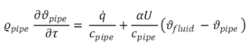
The following equation and set of parameters helps to define a time constant for the mass transfer function:
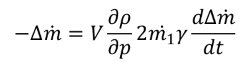 (1) (1) |
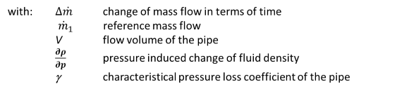
All right hand terms except the differential quotient itself are forming a time constant for the mass storage. Hence it´s becomes possible to integrate this equation by separating the variables and yields directly the transfer function, which represents charge and discharge effects to the stored fluid mass.
The thermal transfer function is derived from the following parameters:
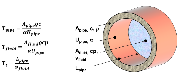 |
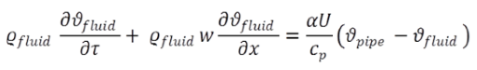 (2) (2) |
 (3) (3) |
These two equations lead combined with the parameters defined above and application of Laplace transformations to the transfer functions representing the thermal behaviour of the component. The following equations show the transfer function for a temperature jump at the inlet of the pipe:
The first right hand sided term mostly could be neglected (due to a value ~1). A transfer back to the time domain is mathematically possible, but not appropriate with respect to the transient EBSILON architecture. Hence a series expansion of the exponential function gives a result, which can be calculated:
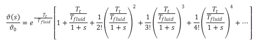 (5) (5) |
Out of this a cascade of coupled PT1-elements weighted by the adequate prefactors can be set up. This substitution gives the transfer function (The ratio Tt/Tfluid is going to be substituted by the expression kD, which is of the same name as the model/calculation approach the method is derived from).
For detailed information please see: B. Epple, R. Leithner, W. Linzer, H. Walter, "Simulation von Kraftwerken und wärmetechnischen Anlagen", Springer Wien New York 2009, p 537fff
 |
Display Option 1 |
Click here >> Component 138 Demo << to load an example.