EBSILON®Professional Online Documentation


|
Line connections |
|
|
|
1 |
Inlet |
|
|
2 |
Outlet |
|
|
P |
Pressure |
|
T |
Temperature |
|
H |
Enthalpy |
|
M |
Mass flow |
|
Q |
Energy Flow |
|
MINREFITP |
Minimum reference value for DITP (optional) - individual specification of the convergence precision for pressure balance equations |
|
MINREFITH |
Minimum reference value for DITH (optional) - individual specification of the convergence precision for enthalpy balance equations |
|
MINREFITM |
Minimum reference value for DITM (optional) - individual specification of the convergence precision for mass balance equations |
For the specification of the material composition and related attributes (net calorific value, density, …) see the chapter "Material Properties".
General Application Example Display Sources & Sinks in Macros Displays Example
The Automatic Connector combines the functionality of EBSILON components to specify stream conditions and composition ( component 1 "Boundary Input Value" or component 33 "General Input Value / Start Value") with the capability to identify ports which should be interconnected (to be identified by a user-defined ID). This functionality allows for creating groups of equipment which can be easily interchanged.
Inlet and outlet ports with identical connector identifier (to be defined in the tab 'Connector') will be connected with a stream of the respective stream type either automatically upon insertion (if the respective option is chosen in the graphics settings under 'General Options - Edit') or with the command 'Edit - Connect open connectors'.
If an automatic connector is connected only on one end, it will behave exactly like component 1 "Boundary Input Value" and it will define the physical properties of the connected stream as entered by the user in the specification values. Once it is connected on both, inlet and outlet port it will neglect these specification values and it will act simply as connecting pipe and stream conditions will be passed through on both ends.
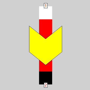
The following description of a simple example shall elaborate on the concept and functionality. Figure 1 shows the model containing a steam source connected to a stream (in the following referred to as ‘stream 1’) and an Automatic Connector as well as a second stream (stream 2’) which originates from another Automatic Connector.
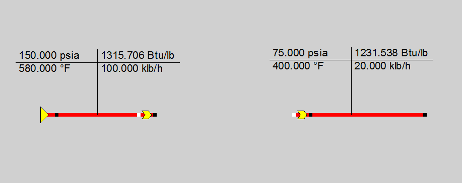
Figure 1: Two steam streams with unconnected Automatic Connectors
Since the Boundary Value and the Automatic Connector of the second stream contain different specifications (see Figures 2 and 4 below), executing the model produces two streams with differing properties. The Automatic Connector connected to the outlet of stream 1 does not contain any specifications and does not contribute to the model calculations. In fact, if it was deleted, the model would produce the exact same result. The purpose of this Automatic Connector is to identify a port to which another Automatic Connector should connect.
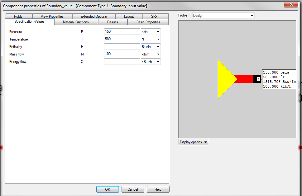
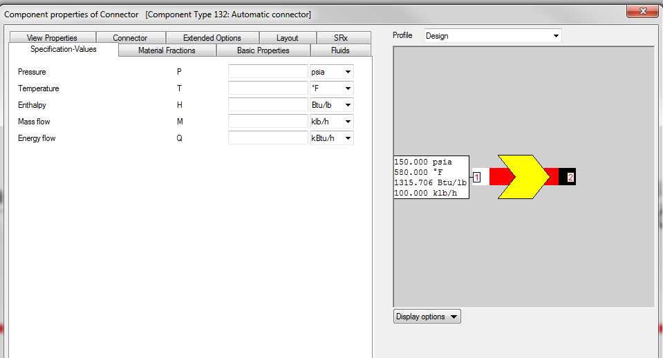
Figure 3: Empty input fields in the Automatic Connector (named ‘Connector’) on stream 1.
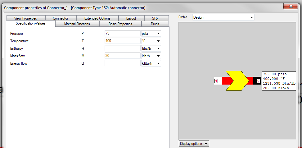
Figure 4: Specifications in the Automatic Connector (named ‘Connector_1’) on stream 2.
In the tab labeled Connector of component 132, the user can define a string which serves as identifier for the Automatic Connector. As can be seen from Figures 5 and 6 below, both Automatic Connectors of the sample model have the string ‘KeyWord’ as Connector-Identifier.
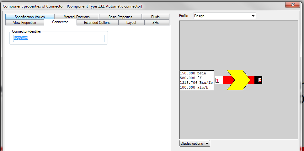
Figure 5: Connector-Identifier in the Automatic Connector (named ‘Connector’) on stream 1.
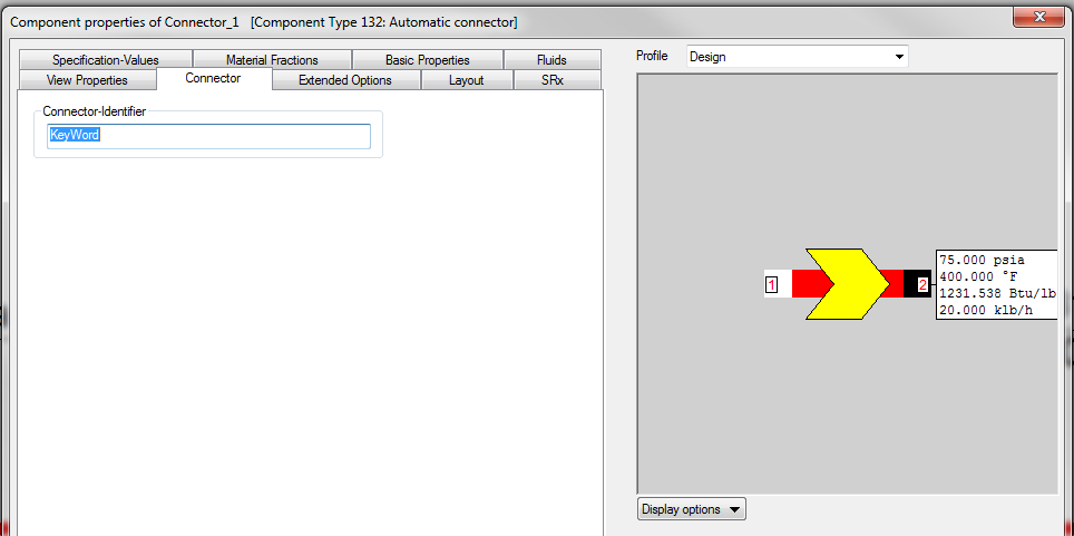
Figure 6: Connector-Identifier in the Automatic Connector (named ‘Connector_1’) on stream 2.
If not specified differently in the general settings of EBSILON, all Automatic Connectors present in a model will connect only upon command which can be triggered from a toolbar icon (see Figure 7) or via the menu item ‘Edit – Connect Open Connectors’.
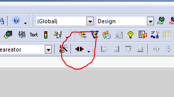
Figure 7: Toolbar icon for connecting open connectors.
Figure 8 below shows the effect of this command on our sample model. Both streams are connected through a third stream that has been inserted between the two Automatic Connectors. If connected on both ends, the Automatic Connector will change to ‘pass-through’ mode in which none of the inputs will be used, so that all of the three streams will have identical data equal to those specified in the Boundary Input Value of stream 1. If the display type '1' has been chosen, the display changes from arrow style to flange style in order to show that the Automatic connector is in ‘pass-through’ mode.
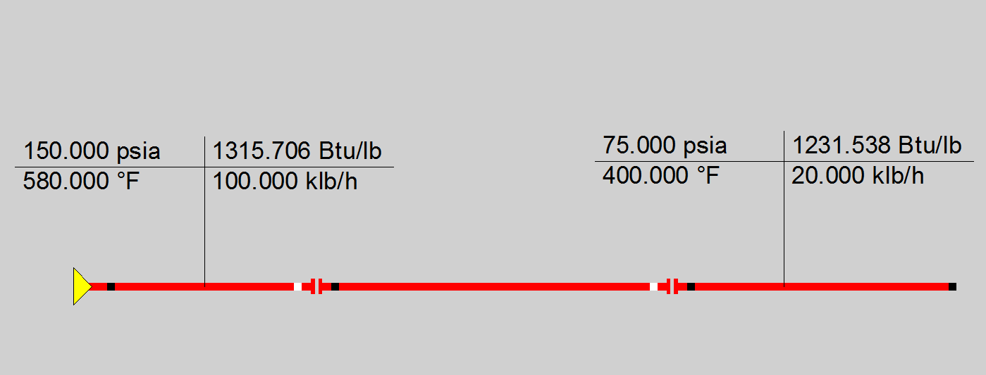
Figure 8: Sample model after pressing ‘Connect Open Connectors’ toolbar icon.
The data in the above figure are not consistent, because the model has not been executed yet. The results after calculation are shown in Figure 9 below.
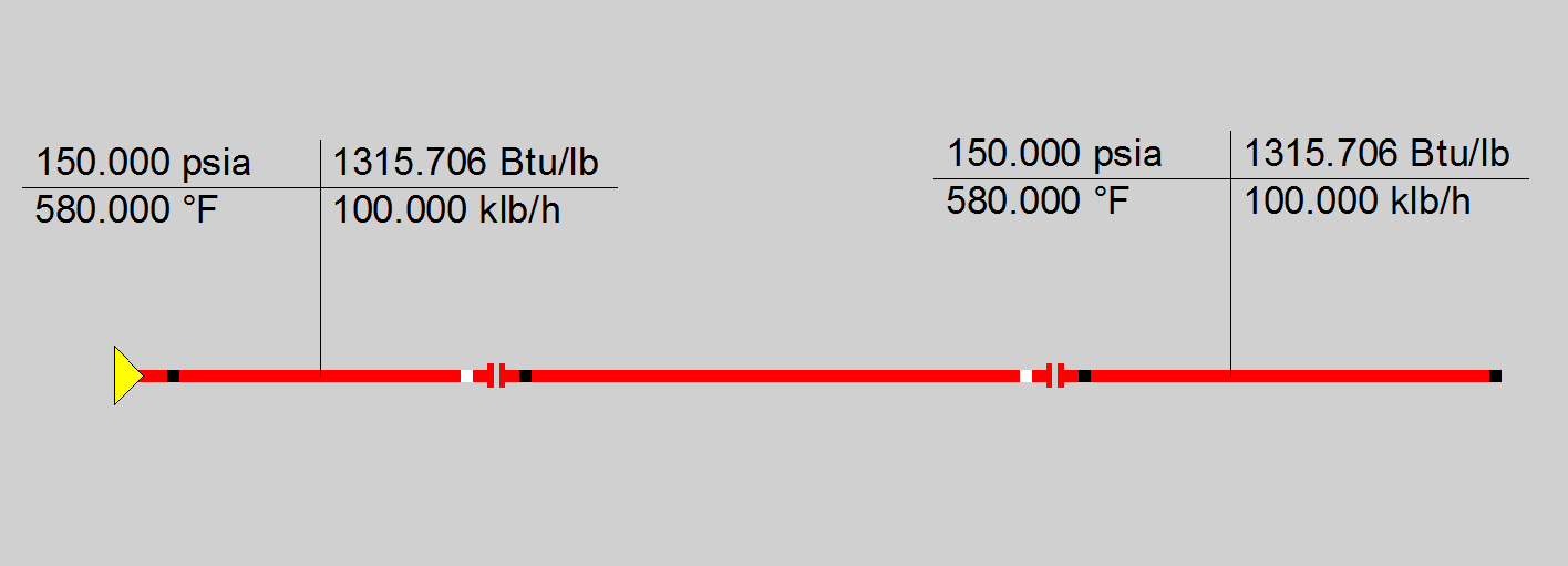
Figure 9: Model results after executing with connected Automatic Connectors
Deleting the new stream will revert the model back to the situation prior to connecting (and thus re-activating Connector_1 as an input component), which upon execution will produce the result as has been shown in Figure 1 above.
As mentioned earlier, the general options of EBSILON also allow for connecting Automatic Connectors immediately when being placed on the flow sheet, if another connector with matching ID exists. This option would speed up the model generation even more, but the user may have less control over the actual routing of the streams than if the routing would be triggered only after the equipment has been placed at the desired location.
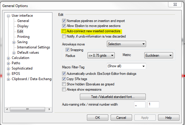
Figure 10: Settings menu for defining options for Automatic Connectors
In case that the command to connect is triggered in a situation where there is more than one possibility for creating a connection (i.e. one outlet port and several inlet ports with the same identifier, or vice versa), than EBSILON will not create the interconnecting stream and the user will have to connect manually until all ambiguities have been resolved.
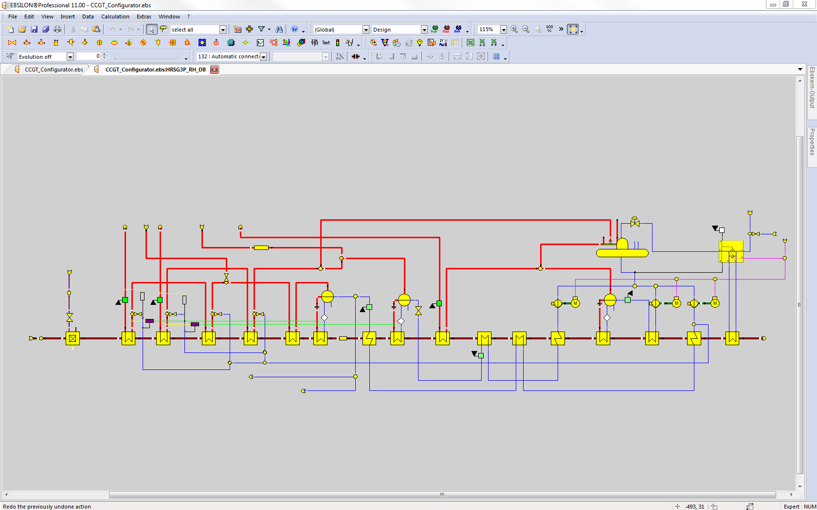
The Automatic Connector may also be used to 'clean up' the display of the content of EBSILON macro objects. By design, all streams that pass through the interface of the macro have to be connected to a port of the macro interface which has a rectangular shape. This leads to a rather busy display of the macro content, as shown in the screen shot below.
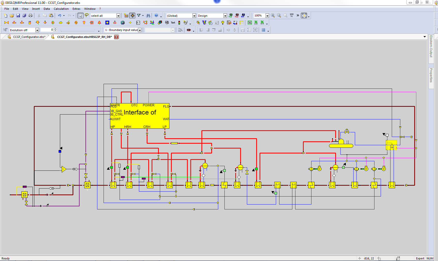
By inserting Automatic Connectors in display mode '2' (which will display the component as arrow even if both ports are connected) at appropriate pipe locations and hiding the macro interface and all pipes that are connected to the interface, the content of the macro can be displayed in the same style as in the calculation sheet.
In Ebsilon the convergence precision is a model-wide setting. It is an upper limit for the admissible relative change of a variable (mass flow, pressure, and enthalpy) from one iteration step
to the next. Only when the relative change in terms of its amount is smaller than this limit for all variables will the iteration procedure be successfully terminated.
Usually this relative change is related to the value of the variable. Thus if e.g. a mass flow changes from 50 to 51 kg/s, the relative change is 1 percent. At a convergence precision of 10-7 (this is the default value) this mass flow of 50 can only change by 0.000005 kg/s more (i.e. 5 mg/s) for this value to be considered convergent. At a mass flow of 0.01 kg/s the admissible change would then only be 10-9 kg/s. Such small changes, however, are not significant in practice and would unnecessarily prolong the iteration. In many cases no convergence could be achieved at all any more due to the “numerical noise“.
For that reason a minimum reference value for calculating the relative change had been defined in Ebsilon. When the value of the variable was smaller than the reference value, the relative change was not calculated with reference to the variable but with reference to the reference value. Thus (at a convergence precision of 10-7) mass flow fluctuations of less than 0.000002 kg/s, pressure fluctuations of less than 0.0000002 bar, and enthalpy fluctuations of less than 0.00006 kJ/kg were no longer considered an obstacle for the conversion.
In Component 1, 33, 132 respectively (boundary, start value, connector respectively) these minimum reference values are specified in the entries
MINREFITP
MINREFITH and
MINREFITM
If these values are left empty, Ebsilon will use the default values. The reference values are then valid for the respective line and are handed down along the main flow.
At a mixer, the reference values of the auxiliary connection (Pin 3) are thus ignored. This facilitates calculating in the sideline with a lower precision while downstream of the mixer, with the main flow, the higher precision applies again.
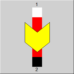 |
Display Options 1 and 2 Remark: Display 1 will automatically switch to display 3, if both, inlet and outlet port are connected. If one of the ports is disconnected again, it will revert back to display style 1. If displays 2 or 3 are selected, the display style will remain the same, independent of the number of connected ports. |
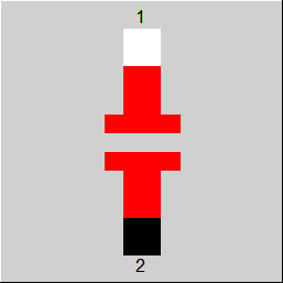 |
Display Option 3 |
Click here >> Component 132 Demo << to load an example.