
EBSILON®Professional Online Documentation


|
Line connections |
||
| Component 1: port 1 | System Boundary |
|
| Component 33: no port number | Connection to line |
|
General User Input Values Results Physic used Display Example
Component 1 is used to define fluid flows that come into the model from outside its boundaries. It represents the starting point of a line. Examples are
Instead, Component 33 can be used for the same purpose, but has to be connected to any line It is recommended and good practice to always define fluids entering the model within a component 1.
It is recommended and is good practice to always define incoming fluids with component 1.
Component 33 differs from component 1 only in its shape: component 1 can only be used at system boundaries, component 33 everywhere. The functionality is exactly the same for both components.
The condition of the fluid is defined by some of the following values:
In case of a setting values (P, H, M) outside of the range of the start and limit values (Model Settings -> Simulation), an error message is issued.
Just three of these five options are enough to describe the condition of the fluid completely. Usually P, T and M are set. H can be calculated from P and T. Q then results from H and M.
Instead of the temperature T, it is also possible to specify the enthalpy H. The temperature T is then calculated from P and H.
If the energy flow Q is specified, the flow rate M is calculated. Also, when the enthalpy H is given. Similarly, if the mass flow M is given, the enthalpy H is calculated.
In some cases, it is not permitted to specify all the three states, since the individual values are known and are already defined at other places of the system. If such a value were set again by a component 1 or 33, this would cause a double definition.
The value entered in the specification value M is multiplied by the specification value LOAD to set the mass flow on a line. This is helpful if you want to calculate different load cases in subprofiles. You then save the calculation of the mass flow in the respective profile and only need to change M in the design profile when copying or changing the default.
The default value for LOAD is 1.0, and as long as you leave LOAD at 1.0 in all profiles, it has no effect.
Attention: For steam in the two-phase area, H must be entered, as P and T are not sufficient to clearly define H.
The specification of the material composition and related attributes (net calorific value, density, …) is described in "Material Properties".
All further information on fluid default values, stream types, material value tables, material value libraries, calorific values, material values, etc. can also be found there.
If you right-click on a numerical value of a composition, there are two further options in addition to the available scaling options:
It should be noted that
The relative humidity can also be specified with a measured value (component 46), but this is not recommended.
By default, the GERG-2008 mechanism is used for mixtures of natural gases, but not for pure fluids. For pure fluids, the equations implemented in REFPROP are more precise as they are not (like in GERG-2008) shortened due to calculation speed. However, the differences are quite small (as long as there is no water in the mixture). The GERG-2008 (developed in Bochum by Wagner and Kunz) offers a higher consistency and precision in the phase equilibrium.
For all fluid libraries assigned to a universal fluid, it is possible to specify a cp correction factor. This is a constant factor by which the specific heat capacity cp and thus also the enthalpy H and the entropy S are multiplied. This can be used in cases where the exact substance data for a particular substance are unknown, but a similar substance is known whose thermodynamic properties can be described accurately enough by adjusting the specific heat capacity at one point.
Note that this correction factor has nothing to do with the default value CPCORR for many other stream types. CPCORR refers exclusively to the ash content in classical fluids (for example, coal and flue gas lines). The cp correction factor available here for the universal fluid, on the other hand, refers to the complete line in the material content table.
In Ebsilon the convergence precision is a model-wide setting. It is an upper limit for the admissible relative change of a variable (mass flow, pressure, and enthalpy) from one iteration step
to the next. Only when the relative change in terms of its amount is smaller than this limit for all variables will the iteration procedure be successfully terminated.
Usually this relative change is related to the value of the variable. Thus if e.g. a mass flow changes from 50 to 51 kg/s, the relative change is 1 percent. At a convergence precision of 10-7 (this is the default value) this mass flow of 50 can only change by 0.000005 kg/s more (i.e. 5 mg/s) for this value to be considered convergent. At a mass flow of 0.01 kg/s the admissible change would then only be 10-9 kg/s. Such small changes, however, are not significant in practice and would unnecessarily prolong the iteration. In many cases no convergence could be achieved at all any more due to the “numerical noise“.
For that reason a minimum reference value for calculating the relative change had been defined in Ebsilon. When the value of the variable was smaller than the reference value, the relative change was not calculated with reference to the variable but with reference to the reference value. Thus (at a convergence precision of 10-7) mass flow fluctuations of less than 0.000002 kg/s, pressure fluctuations of less than 0.0000002 bar, and enthalpy fluctuations of less than 0.00006 kJ/kg were no longer considered an obstacle for the conversion.
Up to Release 11 these minimum reference values were firmly fixed in the code. As of Release 12 it is possible to specify them individually for individual streams. This way, less interesting areas of the model can be calculated with a lower precision, which may reduce the computing time.
In Component 1, 33, 132 respectively (boundary, start value, connector respectively) these minimum reference values are specified in the entries
MINREFITP
MINREFITH and
MINREFITM
If these values are left empty, Ebsilon will use the default values. The reference values are then valid for the respective line and are handed down along the main flow.
At a mixer, the reference values of the auxiliary connection (Pin 3) are thus ignored. This facilitates calculating in the sideline with a lower precision while downstream of the mixer, with the main flow, the higher precision applies again.
Note:
In addition, the feature for the individual specification of the convergence precision implemented in Components 1 and 33 in Release 12 has now been shifted into Component 147. For reasons of compatibility, however, it remains available in Components 1 and 33. The input fields MINREFITP, MINREFITH, and MINREFITM required for this have been hidden but can be rendered visible if required.
Basic Information
Previously it was assumed in Ebsilon that all fluids flow slowly enough so that the kinetic energy can be neglected and total and static state variables can be equated. Therefore no distinction was made between total and static values.
The only exception was the steam turbine (Component 122). As proportionately high flow velocities occur here, the kinetic fractions were considered in the calculation of the steam turbine. In doing so, it was assumed that the variables stored on the lines are total variables as a rule.
Since Release 15, it is now possible to differentiate between total and static variables everywhere. Here the assumption previously made for the steam turbine, namely that the line values are total variables, is applied to all lines.
The conversion between total and static variables requires knowledge of the flow velocity vel (as in Ebsilon the abbreviation v is already used for the specific volume, v is not available for the velocity).
In Ebsilon default units (vel in m/s, H in kJ/kg), the following applies:
Htot = Hstat + Hkin, with
Hkin = 0.0005 * vel²
Here the flow velocity can optionally be specified
In the case of the boundary input value (Component 1) or
the start value (Component 33), the specification is effected by means of one of the specification values VEL_SET, A_SET or D_SET. As a result, all three variables VEL, A, and D will be displayed.
Additionally, the potential energy can be considered in Release 15 as well. The following applies to it in Ebsilon default units (z in m, H in kJ/kg):
Hpot = 0.001 * g * z,
where g = 9.81 m/s² is the acceleration of gravity and z the height, relating to a selected zero level. In Component 1 and 33 respectively, the height is specified by a specification value Z_SET and displayed as result value Z.
Altogether, the following results:
Htot = Hstat + Hkin + Hpot
The distinction between total and static variables only occurs within Component 1 and 33 respectively. It does not make sense to treat the flow velocity as an attribute of the line because the line cross section and thus the flow velocity can change from one position of the line to the next. Therefore the specification and calculation must always be effected together with the specification of the speed (and cross section or diameter respectively).
To allow to observe different flow velocities at various positions of the line, it is possible to set several Components 33 on a line. Specifying static variables, however, is only possible in one component.
If the flow velocity and height respectively is known, the following result values will be displayed in Component 33:
Component 1 and 33 respectively do not only enable the display but also the specification of static state variables. Thus static variables given in thermal flow diagrams or also measured static variables can now be specified this way.
For this – with the exception of the last case – the flow velocity, as described above, must have been specified either directly or via cross section or diameter.
The following options have been implemented:
This case is particularly interesting when static and total pressures are measured by means of various pressure gauges (Prandtl tube, Pitot-Static tube) in order to determine the throughput.
|
State variables for fluids (total. stagnation) |
|
|
P |
Pressure |
|
T |
Temperature |
|
H |
Enthalpy |
|
M |
Mass flow |
| LOAD | Factor for M - the default value is 1.0 |
|
State variables for shafts and electric lines only |
|
|
F |
Frequency/rotary speed (on shafts and electric lines) |
|
Q |
Energy flow (in certain circumstances for other line types as well) |
|
State variables for shafts and electric lines only |
|
|
U |
Voltage (electric lines) |
|
I |
Current (electric lines) |
|
COSP |
Power factor (cos(phi) , phi>0 accepted |
|
PHEL |
Phase shift between voltage and current |
|
NPHAS |
Type of current =0: Direct current |
|
State variables for fluids (static) |
|
|
PSTAT_SET |
Static pressure |
|
TSTAT_SET |
Static temperature |
|
VEL_SET |
Flow velocity |
|
A_SET |
Cross section area |
|
D_SET |
Inner diameter |
|
Z_SET |
Height |
|
Deprecated Settings |
|
|
MINREFITP |
Deprecated (now in component 147): Minimum reference value for DITP |
|
MINREFITH |
Deprecated (now in component 147): Minimum reference value for DITH |
|
MINREFITM |
Deprecated (now in component 147): Minimum reference value for DITM |
|
Fluid composition |
|
|
FFLSET |
Switch to activate the specification of the substance composition (Existing values for the state variables such as P, T, H, M, Q, U, F remain active) 0: Neither composition nor calorific value or fluid coefficients are specified Fluid coefficients are the switches and additional coefficients that are used to calculate the physical properties of classic FDBR fluids (Z factor, ash correction factor, water vapor table, etc.). IntMat mode: Integration of the material equations into the equation system or into the equation matrix - @ calcoptions.sim.intmat = 2 (see model settings -> Simulation -> Iteration) |
|
FMAS |
Content |
|
PHI |
Air humidity (rel.) |
|
FNCV |
Update display for NCV and GCV specification automatically? |
|
FNCVSRC |
Calculation with user-defined input for heating value? |
|
FNCVCALC |
Method used for heating value calculation for gases |
|
TNCVREF |
Reference temperature for calculation of heating value |
|
FNCVCALCELEM |
Method used for heating value calculation for solids (elementary composition C,H,O,N,S,Cl) |
|
NCV |
Net calorific value |
|
GCV |
Gross calorific value |
|
XN2 |
N2- mass fraction |
|
XO2 |
O2- mass fraction |
|
XCO2 |
CO2- mass fraction |
|
XH2O |
Water- mass fraction |
|
XSO2 |
SO2-Massenanteil |
|
XAR |
Argon- mass fraction |
|
XCO |
CO- mass fraction |
|
XCOS |
COS-Massenanteil |
|
XH2 |
H2- mass fraction |
|
XH2S |
H2S- mass fraction |
|
XCH4 |
CH4- mass fraction |
|
XHCL |
HCL-Massenanteil |
|
XETH |
Ethan- mass fraction |
|
XPROP |
Propan- mass fraction |
|
XBUT |
n-Butane- mass fraction |
|
XPENT |
n-Pentane-Massenanteil |
|
XHEX |
n-Hexane- mass fraction |
|
XHEPT |
n-Heptane- mass fraction |
|
XACET |
Azetylen (Ethin, C2H2)- mass fraction |
|
XBENZ |
Benzol (C6H6)- mass fraction |
|
XC |
C mass fraction |
|
XH |
H mass fraction |
|
XO |
O mass fraction |
|
XN |
N mass fraction |
|
XS |
S mass fraction |
|
XCL |
CL mass fraction |
|
XASH |
Ash mass fraction |
|
XLIME |
Lime (Ca(OH)2) mass fraction |
|
XCA |
Elemental calcium mass fraction |
|
XH2OB |
water fraction of fuel |
|
XASHG |
Ash fraction (g) |
|
XNO |
NO-mass fraction |
|
XNO2 |
NO2-mass fraction |
|
XNH3 |
NH3-mass fraction |
|
XMETHL |
Methanol-mass fraction |
|
XMG |
Elemental magnesium mass fraction |
|
XCACO3 |
CaCO3 mass fraction |
|
XCAO |
CaO-mass fraction |
|
XCASO4 |
CaSO4-mass fraction |
|
XMGCO3 |
MgCO3-mass fraction |
|
XMGO |
MgO-mass fraction |
|
XOCT |
n-Octane mass fraction |
|
XNON |
n-Nonane-mass fraction |
|
XDEC |
n-Decane-mass fraction |
|
XDODEC |
n-Dodecane-mass fraction |
|
XIBUT |
Isobutane (2-methylpropane, (CH3)3CH) mass fraction |
|
XIPENT |
Isopentane (2-methylbutane, (CH3)2-CH-CH2-CH3)) mass fraction |
|
XNEOPENT |
Neopentane (2,2-dimethylpropane) mass fraction |
|
X22DMBUT |
Neohexane (2,2-Dimethylbutane, (CH3)2CHCH(CH3)2) mass fraction |
|
X23DMBUT |
2,3-Dimethylbutane ((CH3)2CHCH(CH3)2) mass fraction |
|
XCYCPENT |
Cyclopentane (cyclo-C5H10) mass fraction |
|
XIHEX |
Isohexane (2-methylpentane, (CH3)2-CH-CH2-CH2-CH3) mass fraction |
|
X3MPENT |
3-Methylpentane ((CH3CH2)2CHCH3) mass fraction |
|
XMCYCPENT |
Methylcyclopentane (CH3-C5H9) mass fraction |
|
XCYCHEX |
Cyclohexane (cyclo-C6H12) mass fraction |
|
XMCYCHEX |
Methylcyclohexane (CH3-C6H11) mass fraction |
|
XECYCPENT |
Ethylcyclopentane (C2H5-C5H9) mass fraction |
|
XECYCHEX |
Ethylcyclohexane mass fraction |
|
XTOLUEN |
Toluene (toluol or methylbenzene, C6H5-CH3) mass fraction |
|
XEBENZ |
Ethylbenzene (phenylethane, C6H5-CH2-CH3) mass fraction |
|
XOXYLEN |
ortho-Xylene (1,2-dimethylbenzene, C6H4-2(CH3)) mass fraction |
|
XCDECALIN |
cis-Decalin (decahydronaphthalene) mass fraction |
|
XTDECALIN |
trans-Decalin (decahydronaphthalene) mass fraction |
|
XETHEN |
Ethene (ethylene, C2H4) mass fraction |
|
XPROPEN |
Propene (propylene, C3H6) mass fraction |
|
X1BUTEN |
1-Butene (CH3-CH2-CH=CH2) mass fraction |
|
XC2BUTEN |
cis-2-Butene mass fraction |
|
XT2BUTEN |
trans-2-Butene mass fraction |
|
XIBUTEN |
Isobutene (2-Methylpropene) mass fraction |
|
XIPENTEN |
1-Pentene (C5H10) mass fraction |
|
XPROPADIEN |
Propadiene (allene, CH2=C=CH2) mass fraction |
|
X12BUTADIEN |
1,2-Butadiene (methylallene, CH2=C=CH-CH3) mass fraction |
|
X13BUTADIEN |
1,3-Butadiene (vinylethylene, CH2=CH-CH=CH2) mass fraction |
|
XETHL |
Ethanol mass fraction |
|
XCH3SH |
CH3SH (methanethiol, methylmercaptan) mass fraction |
|
XHCN |
Hydrogen cyanide (prussic acid) mass fraction |
|
XCS2 |
Carbon disulfide mass fraction |
|
XAIR |
Air mass fraction |
|
XHE |
Helium mass fraction |
|
XNE |
Neon mass fraction |
|
XKR |
Krypton mass fraction |
|
XXE |
Xenon mass fraction |
|
XN2O |
Dinitrogen monoxide (laughing gas) mass fraction |
|
VOLA |
Volatile mass fraction |
|
CPCORR |
Correction factor for cp ash |
|
RHOELEM |
Density for fraction defined by elementary analysis |
|
ZFAC |
Z-factor |
|
FSTEAMFORMULATION |
water/steam-formulation |
|
FGASFORMULATION |
gas-formulation |
|
FREALGC |
Real gas correction |
|
FCOAL |
Coal type |
|
SALT |
Mass fraction of salt from total mass |
|
FMED |
Type of medium (only 2-Phase-fluid) |
|
FBIN |
Type of medium (only binary mixture) |
|
XI |
Fraction of refrigerant/anti-freeze medium or water in air |
|
Heating Values |
|
|
NCVI |
Net calorific value (LHV) for 0°C (actual stream value) |
|
VCVC |
Net calorific value (LHV) for 0°C (expected from composition) |
|
GCVI |
Gross calorific value (HHV) for 0°C (actual stream value) |
|
GCVC |
Gross calorific value (HHV) for 0°C (expected from composition) |
|
Depending on velocity and geometry |
|
|
PTOT |
Total pressure |
|
PSTAT |
Static pressure |
|
DPKIN |
Kinetic pressure increase |
|
TTOT |
Total temperature |
|
TSTAT |
Static temperature |
|
DTKIN |
Kinetic temperature increase |
|
HTOT |
Total enthalpy |
|
HSTAT |
Static enthalpy |
|
HKIN |
Kinetic energy |
|
HPOT |
Potential energy |
|
UIE |
Internal energy |
|
HPV |
Displacement energy |
|
RHOTOT |
Total density |
|
RHOSTAT |
Static density |
|
VSTAT |
Static specific volume |
|
VMTOT |
Total volume flow |
|
VMSTAT |
Static volume flow |
|
VEL |
Flow velocity |
|
D |
Inner diameter of tube |
|
A |
Cross section area |
|
MACH |
Mach number |
|
Z |
Height |
|
|
If P is given, then P1=P If H is given, then H1 = H T1 = f(P1, H1) If T is given, then T1 = T H1 = f(P1,T1) If M is given, then M1 = M If Q is given, then Q1 = Q H1=Q1/M1 or M1=Q1/H1 else Q1 = M1*H1 |
|
The five values are only filled with boundary values for the second iteration.
If H1 <= 0 the H1 = f(P1,T1) with specification of P1 and T1
If H1 > 0 then T1 = f(P1,H1) with specification of P1 and H1
If Q1 <= 0 then Q1 = M1 * H1
If Q1 > 0 then H1 = Q1 / M1 if M1 > 0
or M1 = Q1 / H1 if H1 > 0
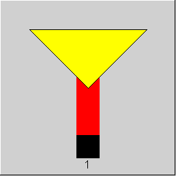 |
Component 1 only display option |
 |
Component 33: display Option 1 component not connected to a pipe |
 |
Component 33: display option 2 component connected to a pipe |
Click here >> Component 1 Demo << to load an example.
Click here >> Component 33 Demo << to load an example.
