EBSILON®Professional Online Documentation


|
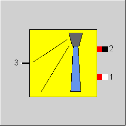
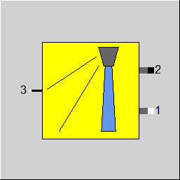
Line Connections |
|
|
|
1 |
Fluid Inlet |
|
|
2 |
Fluid Outlet |
|
|
3 |
Logic connection to heliostat field (121) |
|
General User Input Values Physics Used Characteristic Lines Displays Example
in the solar receiver, the heat flux arriving at the aperture area is transferred into a heat flow directed to the heat transfer medium. There, the heat is used to raise the fluid temperature or, in the case of a steam receiver, the steam fraction. On the way from the aperture to the fluid, some optical and thermal losses occur. These are modelled in the receiver component. The user is free to define the thermal boundary conditions of the model by imposing appropriate values on the connected lines (two quantities of m , Tin and Tout) .
The effective heat (in kW),

transferred to the fluid is determined from

with the heat losses composed of optical, convective and radiation losses,

The optical losses do not depend on the receiver temperature, but convective and radiation heat losses do.
The model offers the user several options how to describe the receiver losses:
• Constant heat loss (model switch FHLOSS=0)
• Constant receiver temperature (model switch FHLOSS=1)
• Variable receiver temperature (model switch FHLOSS=2)
• User defined function for total losses (model switch FHLOSS=3)
• User defined functions for all three loss terms (model switch FHLOSS=4)
• Table based values for total efficiency (FHLOSS=5)
Optical losses
The optical losses are determined from the constant optical efficiency ηopt as
 .
.
This reflects the implementation for options FHLOSS=0, 1, and 2. In case only a total loss term is calculated (FHLOSS=3, 5) the optical losses are set to 0. For FHLOSS=4 a formula for calculation of has to be provided by the user.
Convective losses
For the option “Constant heat losses” (FHLOSS=0), the convective losses are calculated by

with a constant area specific heat loss and the aperture area Arec.
For options 2 and 3 (FHLOSS=2, 3), the convective losses are determined as a function of a mean receiver temperature Trec and a constant heat transfer coefficient Alpha ,

The receiver temperature is either set to a constant value (FHLOSS=2) or calculated from the respective fluid temperature entering, Tin, and leaving, Tout, the receiver.

A weighting factor k for the temperatures is used to allow definition of any representative temperature between inlet and outlet. Over-temperature of the receiver wall outer surface can be expressed by a wall over temperature at design load,  .
.
For option 4 (FHLOSS=4) a user defined function determines the convective heat loss. For options 3 and 5 (FHLOSS=3, 5), only the total loss is represented by either a user-defined function (FHLOSS=3) or a total efficiency approach

by table interpolation (FHLOSS=5). In both cases the convective loss term is used to represent the total loss of the receiver.
An additional user defined function can be used to express wind impact on the convective losses.
Radiation losses
As for the convective heat losses, the radiation losses can be expressed in terms of the mean receiver temperature Trec as

with the emissivity Sigma defined by the user and the Stefan Boltzmann constant Epsilon.
Note that the temperature in EBSILON®Professional is usually given in °C and has to be transformed to K for this calculation. The receiver temperature is either constant (FHLOSS=1) or depends on the inlet and outlet temperature as described above (FHLOSS=2). For options FHLOSS=0, 3, and 5 the radiation losses are set to zero since they are not explicitly considered. In option FHLOSS=4 the user has to provide a function for the radiation heat loss term.
Pressure drop in the receiver
The conventional pressure drop handling of EBSILON®Professional is used also for this component. The user specifies a nominal value and has different options to determine the part load pressure drops.
Interaction between field and receiver
It is important to understand that the heliostat field efficiency matrix is valid only for one configuration. A configuration is defined by the position and parameters of all heliostats in the field as well as the location and extension of the receiver aperture surface. Even an up-scaled, geometrical similar configuration will have a lower field efficiency since distances and, therefore, attenuation of the reflected beams is larger. If the plant is to be erected at another site a new heliostat field should be designed since the optimum heliostat field configuration will be somehow different.
In order to prevent errors by the user all relevant geometrical data for a specific field layout are stored at only one location. This includes total reflective area of heliostat field Arefl , receiver height, receiver radius, receiver view angle, receiver tilt, receiver shape (circular, rectangular, cylindrical, truncated), receiver aperture area Arec (calculated from the quantities above) and tower height.
These variables are stored in the heliostat field component and made available in the receiver component via a connection line. The connection line between is also used to access some thermodynamic variables of the receiver from within the heliostat field model. These are used in the heliostat field model to determine an appropriate focus state.
| FSPEC |
Flag for specifications for mass flow and temperatures =1: Temperatures given, mass flow calculated |
| FHLOSS |
Flag for heat loss model Like in Parent Profile (Sub Profile option only) Expression =0: Constant heat loss =1: Constant receiver temperature (TREC) =2: Variable receiver temperature model =3: Adaptation function for total losses EQLOSS =4: Individual adaptation functions EQLOSSOP, EQLOSSCO, EQLOSSRA =5: Char Lines-based values for total efficiency CQLOSS: ETA(QINC) Note: If option FHLOSS=0 or 1 is chosen, no impact of the fluid temperatures on the heat is considered. |
| ETAOPT | Optical efficiency |
| QALOSS | Aperture specific heat loss (only for FHLOSS==0) |
| EMIS | Emissivity of receiver surface |
| ALPHA | Convective heat loss coefficient |
| TREC | Receiver temperature |
| K | Weighting factor |
| DTWDES | Design wall temperature difference |
| EQLOSS | Adaptation function for all losses a,b,c |
| EQLOSSOP | Adaptation function a for optical losses RQLOSSOP=f(...) |
| EQLOSSCO | Adaptation function b for convection losses RQLOSSCO=f(...) |
| EQLOSSRA | Adaptation function c for radiation losses RQLOSSRA=f(...) |
| FWIND | Method of calculation of wind effects Like in Parent Profile (Sub Profile option only) Expression =0: given by constant factor CORWIND =1: adaptation function EWIND |
| CORWIND | Factor to correct for additional convective heat losses due to wind |
| EWIND | adaptation function for wind impact (result is a factor for convective heat losses) |
| FMODE | Flag for calculation mode Design /Off-design Like in Parent Profile (Sub Profile option only) Expression =0: Global =1: local off-design (i.e. always off-design mode, even when a design calculation has been done globally) =-1: local design |
| DP12N | Nominal pressure loss (this value is used if FDP12N=0) |
| FDP12PL |
Method for calculation of part-load pressure loss Like in Parent Profile (Sub Profile option only) Expression =0: Depending on mass flow =1: Depending on mass and volume flow =2: Constant at nominal value =3: Char Lines-based values CDP12PL: DP12/DP12N=CDP12PL(M1/M1N) =4: Adaptation function EDP12PL: (DP12/DP12N=EDP12PL(M1/M1N)
|
| EDP12PL | for FDP12PL=4 adaptation function part-load pressure drop (DP12/DP12N=EDP12PL(M1/M1N) |
| FQINC |
Definition of incident power Like in Parent Profile (Sub Profile option only) Expression =0: Taken from connected heliostat field module (121) =1: Defined by parameter (for testing purpose) |
| QINC | Incident power on receiver aperture AREC |
| FSTAMB |
Definition of ambient temperature Like in Parent Profile (Sub Profile option only) Expression =0: Given by parameter TAMB =1: Taken from SUN component with index ISUN |
| TAMB | Ambient temperature (this value is used if FSAMB=0) |
| FSWIND |
Definition of wind speed and wind direction Like in Parent Profile (Sub Profile option only) Expression =0: Given by parameters VWIND and AWIND =1: Taken from superior SUN component with index ISUN |
| VWIND | Wind speed (>0, this value is used if FSWIND=0) |
|
AWIND |
Wind direction (from south to north=0°, positive in east direction, values in the range of 0..360°, this value is used if FSWIND=0) |
|
ISUN |
Index of reference solar data component |
|
M1N |
Mass Flow (nominal) |
|
V1N |
Specific Volume at point 1 (nominal) |
The parameters marked in blue are reference quantities for the off-design mode. The actual off-design values refer to these quantities in the equations used.
Generally, all inputs that are visible are required. But, often default values are provided.
For more information on colour of the input fields and their descriptions see Edit Component\Specification values
For more information on design vs. off-design and nominal values see General\Accept Nominal values
| RQINC | Calculated incident power on receiver aperture AREC |
| RQAINC | Calculated specific incident power on receiver =RQINC/AREC |
| QLOSS | Calculated total loss in receiver |
| QALOSS | Calculated specific total loss of receiver =QLOSS/AREC |
| RQLOSSCO | Thermal losses of receiver (convection) |
| RQLOSSRA | Thermal losses of receiver (radiation) |
| RQLOSSOP | Optical losses of receiver |
| RQEFF | Heat absorbed by fluid |
| ETAREC | Receiver efficiency =RQEFF/RQINC |
| RTREC | Effective receiver temperature (if FHLOSS=1,2,[3],[4]) |
| DTW | Wall temperature difference (if FHLOSS=2,[3],[4]) |
| DP12 | Pressure loss |
| RVWIND | Wind speed used in calculation |
| RAWIND | Wind direction used in calculation |
| SCONV | Correction factor for wind impact used in calculation |
| RTAMB | Ambient temperature used in calculation |
| AREC | Receiver aperture area (defined by heliostat field matrix) |
| RECELEV | Height of receiver above ground |
| FRECFORM | Form of receiver |
| RECDIAM | Receiver diameter / width / base diameter |
| RECHEI | Receiver height / diameter / length of edge / length of surface line |
| RECTILT | Receiver tilt angle |
| RECVIEW | Receiver view angle |
| QINCDES | Design intercept power (obtained from heliostat field model) |
The heat input into the fluid flow is given by
| M1*(H2-H1) = RQEFF . |
The effective heat input QEFF depends on the incident power QINC and the losses of the receiver
| RQEFF = RQINC - RQLOSS |
The total heat loss RQLOSS is composed of three single terms
| RQLOSS = RQLOSSOP + RQLOSSCO + RQLOSSRA |
with:
| RQLOSSOP | Optical losses (do not depend on the temperature) |
| RQLOSSCO | Convective heat losses |
| RQLOSSRA | Radiation heat losses |
The user has several options to decide how the loss terms are calculated. These are listed in the following sections:
FHLOSS=0: Constant heat loss
A constant heat loss is prescribed for the absorber in terms of parameters QALOSS. It is not distinguished between radiative and convective heat losses.
| RQLOSSOP | = (1-ETAOPT) * QINC |
| RQLOSSCO | = SCONV * QALOSS * AREC |
| RQLOSSRA | = 0 |
FHLOSS=1: Constant receiver temperature TREC
Radiative (RQLOSSRA) and convective (RQLOSSCO) heat losses are calculated from a prescribed receiver temperature TREC.
| RQLOSSOP | = (1-ETAOPT) * QINC |
| RQLOSSCO | = SCONV * ALPHA * (RTREC - RTAMB) * AREC * 0.001 (W-> kW conversion!) |
| RQLOSSRA |
=EMIS * SIGMA * ( (RTREC+273.15)**4 - (RTAMB+273.15)**4) * AREC * 0.001 (W-> kW conversion!)
with RTREC = TREC SIGMA = 5.6704 E-8 W/(m2K4) (Stefan-Boltzmann constant) |
FHLOSS=2: Variable receiver temperature
This option is similar to FHLOSS=1, but the receiver temperature is determined from the fluid inlet (T1) and outlet (T2) temperatures of the receiver. The user has the possibility to define the weighting between inlet and outlet temperature via parameter K. In addition, a load depended temperature across the receiver wall is added. The user has to specify the design temperature difference DTWDES and the design incident power QINCDES (restricted specification value).
| RQLOSSOP | = (1-ETAOPT) * QINC |
| RQLOSSCO | = SCONV * ALPHA * (RTREC - RTAMB) * AREC * 0.001 (W-> kW conversion!) |
| RQLOSSRA |
=EMIS * SIGMA * ( (RTREC+273.15)**4 - (RTAMB+273.15)**4) * AREC * 0.001 (W-> kW conversion!)
with RTREC = T1 + K * ( T2 - T1 ) + DTWDES * QINC / QINCDES SIGMA = 5.6704 E-8 W/(m2K4) (Stefan-Boltzmann constant) |
FHLOSS=3: Adaptation function for total losses
The user may provide an adaptation function EQLOSS for the total receiver losses (including optical!). This option is intended for the user who wants to provide a rather comprehensive receiver loss model with strong interaction between the loss terms.
| RQLOSSOP | = 0 |
| RQLOSSCO | = SCONV * EQLOSS() |
| RQLOSSRA | = 0 |
FHLOSS=4: Individual adaptation functions for losses
The user may provide individual adaptation functions for the three loss terms. This is useful if the three terms can be calculated more or less independent from each other.
| RQLOSSOP | = EQLOSSOP() |
| RQLOSSCO | = SCONV * EQLOSSCO() |
| RQLOSSRA | = EQLOSSRA() |
FHLOSS=5: Char Lines-based values for total efficiency
This option is intended for the user who knows a load depended efficiency curve of the receiver.
| RQLOSSOP | = 0 |
| RQLOSSCO | = SCONV * CQLOSS * QINC |
| RQLOSSRA |
= 0
with CQLOSS = CQLOSS (QINC/QINCDES) |
Thermal losses of the receiver might be higher with wind (forced convection). A multiplier SCONV is introduced to model the increased convective heat loss RQLOSSCO. The factor SCONV is calculated as
| FWIND=0: | SCONV = CORWIND |
|
FWIND=1: |
SCONV=CORWIND*EWIND
(wind influence can be modelled in adaptation function EWIND, default for EWIND is 1) |
where CORWIND is a parameter >=1 and EWIND is an adaptation function with a result value >=1.
The conventional pressure drop handling of EBSILON®Professional is used also for this component. The user specifies a nominal value and has different options to determine the part load pressure drops.
The nominal pressure loss has to be prescribed by the user via parameter DP12N
The user has the following options for the calculation of the part-load pressure loss:
|
FDP12PL=0: |
Dependent on mass flow (in relation to nominal values) |
|
FDP12PL=1: |
Dependent on mass and volume flow (in relation to nominal values) |
|
FDP12PL=2: |
Constant at nominal value |
|
FDP12PL=3: |
Char Lines-based values CDP12PL: DP12/DP12N=CDP12PL(M1/M1N) |
|
FDP12PL=4: |
Adaptation function EDP12PL: (DP12/DP12N=EDP12PL(M1/M1N) |
CD12PL: Pressure loss characteristic
DP12/DP12N = f(M1/M1N)
CQLOSS: Heat loss characteristic
QLOSS/QINC = f(QINC/QINCDES)
 |
Display Option 1 |
Click here >> Component 120 Demo << to load an example.-