Component 116: Solar Field

In This Topic

Component 116: Solar Field

Specifications

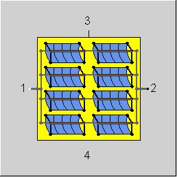
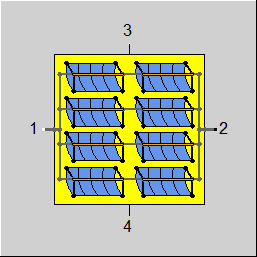
Line connections
1	Fluid inlet
2	Fluid outlet
3	Limit input
4	Logic outlet

General User Input Values Physics Used Characteristic Lines Displays Example

General

The solar field model can be used to simulate the performance of a whole solar field. The size of the field is determined by the number of collectors NCOLL and the data of the collector model. Calculation methods are nearly identical to the ones in the collector component 113. Additional terms are available to describe the kind of process in the field and the heat losses of the interconnecting and header piping. In contrast to the collector component model based pressure loss calculation is not available here since the pressure loss strongly depends on the detailed layout of the field which is in the end an economic factor. The user may use the collector component 113 in conjunction with the header components 114 and 115 to determine the pressure loss for a specific field design.

Like in the case of component 113 (Linear Focusing Solar Collector), the polynomial for calculating the heat losses has been enhanced and a logic outlet for QEFF has been added, too.

User Input Values

Process parameters

FPROC

Type of the process

Like in Parent Profile (Sub Profile option only)

Expression

=0: Sensible (liquid or gas)

=1: Pre-heating and evaporation

=2: Pre-heating, evaporation and super heating

FSPEC

Calculation method

Like in Parent Profile (Sub Profile option only)

Expression

=0: Mass flow predefined, outlet state calculated

=1: Outlet state predefined, required mass flow calculated

Geometric Parameters

COLSET	Collector set load
FTYPE	Collector type Like in Parent Profile (Sub Profile option only) Expression =0: Parabolic trough =1: Linear Fresnel
LENGTH	Gross length of one collector unit
AWIDTH	Gross aperture width of one collector unit
NRATIO	Ratio of active reflective area to gross collector area given by LENGTH*AWIDTH
LFOCAL	Focal length of collector (parabolic trough), height of absorber tube over mirror plane (Linear Fresnel) (used for end loss calculation)
ROWDIST	Distance of the axis of two parallel collector rows (used for shading calculation)
CDIST	Distance between two collectors in series (used for calculation of end gains if FELOSS=2..4)
CAZIM	Collector azimuth angle: Direction of the positive collector axis. Towards north=0°, positive in eastern direction (used for calculation of incident and transversal angle if FSPHI=2)
CSLOP	Collector axis slope: Angle between collector axis and horizontal plane (used for calculation of incident and transversal angle if FSPHI=2)
NCOLL	Number of collector units in the field
FMODE	Flag for calculation mode =0: Global =1: local off-design (i.e. always off-design mode, even when a design calculation has been done globally) = -1: local design

Pressure Loss Parameters

DP12N	Nominal pressure loss
FDP12PL	Method for calculation of part-load pressure loss Like in Parent Profile (Sub Profile option only) Expression =0: Depending on mass flow =1: Depending on mass and volume flow =2: Constant at nominal value (calculated according to FDP12N) =4: Adaptation function EDP12PL Indexing chosen to be consistent with component 113 (solar collector)
DPSHN	Nominal pressure loss of super heater (only if FPROC=2)
EDP12PL	for FDP12PL=4 adaptation function part-load pressure drop in relation to nominal pressure drop.

Performance Parameters

FOPT0	Peak optical efficiency (related to the net aperture area LENGTHAWIDTHNRATIO)
CLEANI	Cleanliness of the mirrors as a ratio of actual reflectivity to nominal reflectivity assumed for FOPT0 (standard value is 1 indicating clean mirrors)
AVAIL	Actual field availability
CORSHAD	Factor to tune the result of the shading model (1=no correction of model)
FELOSS	Method for calculation of optical end losses and end gains Like in Parent Profile (Sub Profile option only) Expression =0: Optical end losses not considered (also end gains not considered) =1: End losses considered according to model and tuning factor CORELOS =4: End losses and end gains at both sides of collector considered according to model and tuning factors CORELOS and COREGAI are used (index 4 chosen to remain consistent with Component 113)
CORELOS	Factor to tune the optical end losses calculated from the end loss model (1=no correction of model)
COREGAI	Factor to tune the optical end gains calculated from the end gain model (1=no correction of model)
FWIND	Tuning factor for wind impact (1=no correction) Like in Parent Profile (Sub Profile option only) Expression =0: Given by factor CORWIND =1: Adaptation function EWIND
CORWIND	Factor to describe wind impact on optical performance (1=no impact or impact defined by EWIND)
EWIND	for FWIND=1 adaptation function wind impact: Result: 0..., default is 0.
XEVAP	Steam fraction at outlet of evaporator (used for receiver heat loss calculation if FPROC=2 is chosen)
FPIPELOSS	Model for heat losses of interconnecting and header piping Like in Parent Profile (Sub Profile option only) Expression =0: Constant value defined by parameter PIPELOSS =1: Temperature dependent (nominal state given by parameter PIPELOSS) =2: Defined by adaptation function EPIPELOSS
PIPELOSS	Nominal heat loss of all solar field piping except of receivers (refers to net aperture area)
EPIPELOSS	for FPIPELOSS=2 adaptation function for piping heat losses. Result: W/m**2

Power Limitations

These specification values for power limitation are used if definition by specification value is chosen in FLIMITS (=0). Otherwise (FLIMITS=1) the corresponding values are read from line "3".

FLIMIT	Method for limitation of power Like in Parent Profile (Sub Profile option only) Expression =0: Focus state predefined (FOCUS) =1: Limitation of mass flow (M2MIN, M2MAX) - used only if mass flow calculation is chosen (FSPEC=1) =2: Limitation of thermal power (QMAX) - used only if mass flow calculation is chosen (FSPEC=1) =3: Limitation of outlet temperature (T2MAX) - used only if outlet state calculation is chosen (FSPEC=0) =4: Limitation of outlet specific enthalpy (H2MAX) - used only if outlet state calculation is chosen (FSPEC=0) =5: Limitation of outlet steam fraction (X2MAX) - used only if outlet state calculation (FSPEC=0) in combination with evaporation process (FPROC=1) is chosen
FLIMITS	Method for definition of limiting value Like in Parent Profile (Sub Profile option only) Expression =0: Limit is defined by a specification value. This is either FOCUS, M2MAX, QMAX, T2MAX, H2MAX or X2MAX, according to choice of FLIMIT =1: Limit is defined by the logical line at port 3. The choice of FLIMIT determines which property of this line is used: In case of "limitation of mass flow" the mass flow property of the line is used In all other cases, the enthalpy property of the line is used. In this case, it is possible to put a measurement value on of the requested (according to FLIMIT) type on the logical line. This is possible, because EBSILON^®Professional uses a definition for heat flow, temperature and steam content on logical lines where the value of this properties is equal to the value of the enthalpy
FOCUS	Focus state of the collector (0=not focused, 1=focused, linear in between, used if FLIMIT=0)
M2MIN	Minimum mass flow (used if FSPEC=1 and FLIMIT=1)
M2MAX	Maximum mass flow (used if FSPEC=1 and FLIMIT=1)
QMAX	Maximum thermal power of field (used if FSPEC=1 and FLIMIT=2)
T2MAX	Maximum outlet temperature (used if FSPEC=0 and FLIMIT=3 and FPROC=0/2)
H2MAX	Maximum outlet specific enthalpy (used if FSPEC=0 and FLIMIT=4)
X2MAX	Maximum outlet steam fraction (used if FSPEC=0 and FLIMIT=3 and FPROC=1)

Ambient and Irradiance Parameters

FSPHI	Definition of incident and transversal angle Like in Parent Profile (Sub Profile option only) Expression =0: Given by parameters PHIINC and PHITRAN =1: Incident and transversal angle taken from calculation in superior SUN component with index ISUN =2: Incident and transversal angle calculated from collector orientation (given by parameters CAZIM and CSLOP) and sun position obtained from superior SUN component with index ISUN
PHIINC	Incident angle prescription (this value is used if FSPHI=0)
PHITRAN	Transversal angle prescription (this value is used if FSPHI=0)
FSDNI	Definition of direct normal irradiance Like in Parent Profile (Sub Profile option only) Expression =0: Given by parameter DNI =1: Taken from superior SUN component with index ISUN
DNI	Direct normal irradiance (this value is used if FSDNI=0)
FSTAMB	Definition of ambient temperature Like in Parent Profile (Sub Profile option only) Expression =0: Given by parameter TAMB =1: Taken from superior SUN component with index ISUN
TAMB	Ambient temperature (this value is used if FSAMB=0)
FSWIND	Definition of wind speed and wind direction Like in Parent Profile (Sub Profile option only) Expression =0: Given by parameters VWIND and AWIND =1: Taken from superior SUN component with index ISUN
VWIND	Wind speed (>0, this value is used if FSWIND=0)
AWIND	Wind direction (from south to north=0°, positive in east direction, values in the range of 0..360°, this value is used if FSWIND=0)
ISUN	Index of reference solar data component (component 117)

Incident angle correction

FIAM	Method for calculation of incident angle correction Like in Parent Profile (Sub Profile option only) Expression =0: Standard polynomial =1: Adaptation functions defined in EPHIINC and EPHITRAN =2: Table based values given by CIAMINC and CIAMTRAN
IAMLA	Coefficient for standard formulation (longitudinal)
IAML0	Coefficient for standard formulation (longitudinal)
IAML1	Coefficient for standard formulation (longitudinal)
IAML2	Coefficient for standard formulation (longitudinal)
IAML3	Coefficient for standard formulation (longitudinal)
IAML4	Coefficient for standard formulation (longitudinal)
IAML5	Coefficient for standard formulation (longitudinal)
IAMLCOS	Coefficient for standard formulation (longitudinal)
IAMT0	Coefficient for standard formulation (transversal)
IAMT1	Coefficient for standard formulation (transversal)
IAMT2	Coefficient for standard formulation (transversal)
IAMT3	Coefficient for standard formulation (transversal)
IAMT4	Coefficient for standard formulation (transversal)
IAMT5	Coefficient for standard formulation (transversal)
IAMTCOS	Coefficient for standard formulation (transversal)
EPHIINC	for FIAM=1 adaptation function for incident angle. Result: 0...90°
EPHITRAN	for FIAM=1 adaptation function for transversal angle. Result: 0...90° or 270°...360°)

Heat loss parameters

FQLOSS	Method for heat loss calculation Like in Parent Profile (Sub Profile option only) Expression =0: Standard polynomial =1: Adaptation function defined in EQLOSS =2: Table based values given by QLOSSA and QLOSSB
QLOSSA0	Coefficient for standard formulation heat loss (no DNI dependency) (constant Term in dT) (for FQLOSS=0)
QLOSSA1	Coefficient for standard formulation heat loss (no DNI dependency) (linear Term in dT) (for FQLOSS=0)
QLOSSA2	Coefficient for standard formulation heat loss (no DNI dependency) (^2 Term in dT) (for FQLOSS=0)
QLOSSA3	Coefficient for standard formulation heat loss (no DNI dependency) (^3 Term in dT) (for FQLOSS=0)
QLOSSA4	Coefficient for standard formulation heat loss (no DNI dependency) (^4 Term in dT) (for FQLOSS=0)
QLOSSB0	Coefficient for standard formulation heat loss (DNI dependency) (const. Term in dT) (for FQLOSS=0)
QLOSSB1	Coefficient for standard formulation heat loss (DNI dependency) (lin. Term in dT) (for FQLOSS=0)
QLOSSB2	Coefficient for standard formulation heat loss (DNI dependency) (^2 Term in dT) (for FQLOSS=0)
QLOSSC1	Coefficient for standard formulation heat loss (no DNI dependency) (lin. Term in T) (for FQLOSS=0)
QLOSSC2	Coefficient for standard formulation heat loss (no DNI dependency) (^2 Term in T) (for FQLOSS=0)
QLOSSC3	Coefficient for standard formulation heat loss (no DNI dependency) (^3 Term in T) (for FQLOSS=0)
QLOSSC4	Coefficient for standard formulation heat loss (no DNI dependency) (^4 Term in T) (for FQLOSS=0)
QLOSSD1	Coefficient for standard formulation heat loss (DNI dependency) (lin. Term in T) (for FQLOSS=0)
QLOSSD2	Coefficient for standard formulation heat loss (DNI dependency) (^2 Term in T) (for FQLOSS=0)
EQLOSS	for FQLOSS=1 adaptation function for receiver heat losses. Result: [W/m]

Nominal parameters

M1N	Mass flow (nominal)
VREFN	Specific volume at reference point (nominal)
T1N	Inlet temperature (nominal)
T2N	Outlet temperature (nominal)

The parameters marked in blue are reference quantities for the off-design mode. The actual off-design values refer to these quantities in the equations used.

Generally, all inputs that are visible are required. But, often default values are provided.

For more information on colour of the input fields and their descriptions see Edit Component\Specification values

For more information on design vs. off-design and nominal values see General\Accept Nominal values

Result values

RDNI	Direct normal irradiance used for calculation
RSHEIGHT	Sun height angle used for calculation
RSAZIM	Sun azimuth angle used for calculation
RPHIINC	Incident angle used for calculation
RPHITRAN	Transversal angle used for calculation
ETAOPT	Optical efficiency RFOCUS * QSOLAR / (DNI * ANET)
ETATHERM	Thermal efficiency QEFF / RFOCUS * QSOLAR
ETAFIELD	Field efficiency ETAOPT * ETATHERM
QSOLAR	Solar power on absorbers
QLOSS	Heat losses of absorbers
QPIPE	Heat losses of the field piping
QEFF	Heat absorbed by fluid
QAVAIL	Available heat input
RFOCUS	Focus state used for calculation
AGROSS	Total gross aperture area
ANETCOLL	Net aperture area of one collector
ANET	Total net aperture area
QASOLAR	Area specific solar heat QSOLAR / ANET
QALOSS	Area specific receiver heat losses QLOSS / ANET
QAPIPE	Area specific piping losses QPIPE / ANET
QAEFF	Area specific effective heat QEFF / ANET
QLSOLAR	Length specific solar heat QSOLAR / (LENGTH*NCOLL)
QLLOSS	Length specific receiver heat losses QLOSS / (LENGTH*NCOLL)
QLPIPE	Length specific piping losses QPIPE / (LENGTH*NCOLL)
QLEFF	Length specific effective heat QEFF / (LENGTH*NCOLL)
KIA	Incident angle modifier
KIAINC	Incident angle modifier (longitudinal part)
KIATRAN	Incident angle modifier (transversal part)
ETASHAD	Shading efficiency
ETAENDL	Endless efficiency
ETASPILL	Spillage efficiency
DP12	Pressure loss over collector
DPSH	Superheated pressure loss
RVWIND	Wind speed used in calculation
RAWIND	Wind direction used in calculation
RTAMB	Ambient temperature used in calculation
RPH	Fraction of pre-heating
REV	Fraction of evaporation
RSH	Fraction of super heating

Physics used

Equations

Calculation method

The user has to select between two principle calculation modes (FSPEC)

FSPEC=0: The mass flow is predefined by the user (via line 1 or 2), the model calculates the outlet state under the actual ambient conditions.
FSPEC=1: The desired outlet state is predefined, the model calculates the required mass flow.

General heat balance

The heat input into the fluid flow is given by

M1*(H2-H1) = QEFF .

This equation is used for both parabolic trough and Linear Fresnel collector fields and all types of processes (sensible or latent/sensible). The available heat input QAVAIL depends on the solar heat input QSOLAR and the thermal losses of the receivers QLOSS and the field piping QPIPE

QAVAIL = QSOLAR - QLOSS - QPIPE .

Due to limited capacities of heat consumption the solar field will often not use all of the available solar energy. Parts of the fields will be defocused. The effective heat generated in the solar field is therefore reduced by the fraction which is lost due to defocused collectors

QEFF = QSOLAR * RFOCUS - QLOSS - QPIPE

where RFOCUS is the actual focus state of the collector field. This value is determined by the selected power limitation method FLIMIT and is described in a separate paragraph. It is assumed that the heat losses are present although parts of the field are not focused.

The solar input QSOLAR is determined by the equation

QSOLAR = DNI * ANET * FOPT_0 * KIA * ETASHAD * ETAENDL * ETASPILL * ETA_CLEAN * AVAIL

with the terms:

DNI Direct normal irradiance in W/m**2

ANET Net aperture area ANET=NCOLL*LENGTH*AWIDTH*NRATIO

FOPT_0 Peak optical efficiency (parameter FOPT0)

KIA Incident angle correction (cosine losses already included)

ETASHAD Factor to include shading losses

ETAENDL Factor to correct end loss effects determined from model

ETASPILL Factor to include optical losses due to wind impact

ETA_CLEAN Factor to correct for actual mirror cleanliness ETA_CLEAN=CLEANI

AVAIL Field availability

Compared to the component 113 (Linear Focusing Solar Collector) this equation does not contain the FOCUS parameter since the focus impact is defined at another point. In addition the AVAIL occurs.

The heat losses of the collector to the surrounding are calculated based on the length-specific heat loss qloss by

QLOSS = qloss * LENGTH * NCOLL

The applied methods for the calculation of the terms are provided in the following section.

Important hints for the user:

The performance of the collector depends on the product

FOPT0 * LENGTH * AWIDTH * NRATIO .

Since performance data found in literature do not have a unique structure please make sure that FOPT0 is always used together with the corresponding reference area. This might be the gross area as given by LENGTH*AWIDTH or the net area which is reduced by factor NRATIO. If the gross area is reported as the reference, NRATIO should be equal to 1 to come to correct results.

For Linear Fresnel systems AWIDTH is considered as the width of the collector system. Due to the facetted structure NRATIO is used to define the net aperture area. It is in the choice of the manufacturer if the net aperture area is defined as the area if all facettes are looking to the zenith or the one of the projected area at perpendicular irradiation. For correct results the aperture area definition should be consistent with the peak optical efficiency value and the incident angle correction values KIA.

For linear Fresnel systems the peak optical efficiency might not be reached at perpendicular irradiance due to the specific optics of these systems. Two options for defining the parameters are open to the user:

Option 1: Define the peak optical efficiency as the optical efficiency reached at PHIINC=0. Then, for Fresnel systems, the incident angle modifier KIA will result in 1 at PHIINC=0 and PHITRAN=0 and might reach values >1 for PHIINC<>0.
Option 2: Define the peak optical efficiency as the peak value reached over the whole range of PHIINC, PHITRAN. Then, the incident angle modifier KIA will be smaller than 1 at PHIINC=0, PHITRAN=0 and 1 for the combination of PHIINC and PHITRAN where the peak optical efficiency is reached.

Solar input: QSOLAR

The peak optical efficiency FOPT0 describes the optical efficiency of the collector under the assumptions

no heat losses to the surrounding (fluid temperature is the same as ambient temperature)
sun beam hits the aperture area perpendicular (incident angle is 0).
mirrors are ideally clean so that they reach their peak reflectivity (the value of which is included in FOPT0)
the collector is focused
no deformation of the collector structure due to wind
no shading of parallel collector rows occurs (sun is high above horizon)

Deviations from this ideal reference point are described by a number of factors that reduce the available heat. These are described in the following.

Incident angle correction: KIA (equal to component 113)

At non-perpendicular incident of the sun, additional losses due to shading of collector structure elements, a longer optical path of the reflected sun rays and angle-dependent optical properties of mirrors and absorber tube occur. These optical effects are summarized in the incident angle correction KIA. Note that this factor already includes the cosine losses of the parabolic trough collector in order to allow the same methodology as for Linear Fresnel systems.

The incident angle correction KIA is calculated as

KIA = KIAINC(RPHIINC) for parabolic trough systems,

KIA = KIAINC(RPHIINC) * KIATRAN(RPHITRAN) for Linear Fresnel systems,
with RPHITRAN=abs(PHITRAN).

The user has three options to specify the relations between the angles RPHIINC, RPHITRAN and KIAINC and KIATRAN which are chosen by flag FSPHI.

FIAM=0: defined by the standard functions with parameters IAMxx
FIAM=1: given by user-defined functions EPHINC and EPHITRAN
FIAM=2: given by characteristic lines CIAMINC and CIAMTRAN

The standard function for parabolic troughs is defined as

KIAINC = ( 1-IAMLA+IAMLA*cos(RPHIINC) ) * (IAMLCOS*cos(RPHIINC) + IAMLO + IAML1*RPHIINC + IAML2*RPHIINC**2 + IAML3*RPHIINC**3 + IAML4*RPHIINC**4 + IAML5*RPHIINC**5 )

The structure of this function is chosen to be able to represent common formulations from literature. The terms in the first bracket are necessary if a polynomial-based relation for the incident angle correction has to be represented which does not already include the cosine of the incident angle.

For the Linear Fresnel system the correlations

KIAINC = IAMLO + IAML1*RPHIINC + IAML2*RPHIINC**2 + IAML3*RPHIINC**3 + IAML4*RPHIINC**4 + IAML5*RPHIINC**5

KIATRAN = IAMTO + IAMT1*RPHITRAN + IAMT2*RPHITRAN**2 + IAMT3*RPHITRAN**3 + IAMT4*RPHITRAN**4 + IAMT5*RPHITRAN**5

are used. In all cases the results of the functions are limited to a minimum value of 0. When using the adaptation function or table based method always check if the units (deg or rad) of RPHIINC, RPHITRAN fit to the values you specify.

Shading losses: ETASHAD (equal to component 113)

If the sun is near the horizon parallel collector rows shade each other. This effect is considered by means of the term ETASHAD which is calculated based on geometric relation in dependence of the track angle (=transversal angle) of parabolic trough systems.

ETASHAD=1 - min(1, CORSHAD * max( 0,1- ROWDIST * cos(RPHITRAN) / AWIDTH ) )

The term min(...) describes the reduction of available energy as a fraction of the energy available if no shading occurs. If the sun is high above the horizon this term equals to 0 and the ETASHAD is 1. The user has the possibility to tune the model based shading effect by a tuning factor CORSHAD.

The calculation above assumes that each collector row has a neighbouring row at both sides. In a real solar field this is not true at the borders. Thus, the shading losses can be slightly reduced by choosing a CORSHAD value smaller than 1.

Optical end loss effects: ETAENDL (similar to component 113)

At incident angles <>0 some fraction of the reflected sun beams at the ends of the collector do not hit the absorber tube. This effect is called optical end loss and is a function of the incident angle RPHIINC. If the next collector is arranged in the same axis the lost sun beams of one collector can hit the absorber tube of the next collector. A fraction of the lost heat can be therefore be regained. This effect is called optical end gain. Since a collector can have a corresponding neighbour collector at one side or at both sides, the effective end gains depend on the position of the collector in the field. Due to symmetry reasons the field averaged end gains are assumed to be not dependent on the position of the sun relative to the collector axis. The user has to specify via parameter CORELOS to which extend end losses are available in the current solar field design. The flag FELOSS defines in which way the end effects are handled:

FELOSS=0: Optical end losses are not considered (also end gains are not considered).
FELOSS=1: End losses are considered according to geometric model and a tuning factor CORELOS.
FELOSS=2: due to averaging effects over the field not considered in this component.
FELOSS=3: due to averaging effects over the field not considered in this component.
FELOSS=4: End losses and end gains at both sides of the collector are considered according to geometric model and tuning factors CORELOS and COREGAI.

The end loss effects ETA_ELOS are calculated based on the equation

ETA_ELOS =1

- CORELOS * min(1, kel * LFOCAL/LENGTH * tan(RPHIINC) )

+ COREGAI * max( 0, keg*min(1, kel * LFOCAL/LENGTH * tan(RPHIINC) ) - CDIST/LENGTH )

where the term with CORELOS represents the end losses and the term with COREGAI represents the end gains. The parameters CORELOS and COREGAI are tuning factors with a default value of 1 that correct the calculated effects by a factor. The values kel and keg are used to include the user's choice in flag FELOSS:

FELOSS=0: kel=0; keg=0
FELOSS=1: kel=1; keg=0
FELOSS=4: kel=1, keg=1.

For the calculation based on FELOSS=2, 3 the sun position (azimuth angle SAZIM) is required to determine the sun position relative to the collector. The sun position has to be provided by the sun model with index ISUN. For the other options the sun position is not required to calculate the end losses.

If CORELOS is equal to 1 end gains are generated at each collector in the field. This is true for an infinitesimal number of collectors and all collectors are arranged in series along one single axis. For a more realistic solar field with for example four collector loops in a row and a U-type arrangement of the four collectors end gains can only be obtained at two of the three collectors. Thus, the user should specify COREGAI=0.5 . If an additional correction beyond this "solar field arrangement" factor is required, the COREGAI can be further reduced.

Wind effects on optical performance: ETASPILL (equal to component 113)

Under wind loads the collector structure is deformed which reduces the optical efficiency. This effect is represented by the factor ETASPILL. There is no model or standard formulation for the spillage effect included since data on this effect are sparse. The user has two possibilities:

FWIND=0: constant factor that reduces available heat ETASPILL = CORWIND * 1 (no influence of actual RVWIND)
FWIND=1: Adaptation function ETASPILL = 1 - CORWIND * min(1, EWIND) (wind influence can be modelled in adaptation function EWIND, default for EWIND is 0)

Cleanliness of mirrors: ETA_CLEAN (equal to component 113)

The actual cleanliness of the mirrors relative to the ideally clean state can be specified by parameter CLEANI so that ETA_CLEAN=CLEANI.

Field Availability: AVAIL (in addition to component 113)

This factor is intended to include a user-defined availability of the field which might be caused by revision works or degradation over a long period.

Heat losses of the receiver: QLOSS

Due to a temperature difference between the heat transfer fluid and the ambient air, heat losses occur in the collectors of the field. Heat losses are assumed to only depend on the temperature difference. Compared to the collector component 113 there may be a large temperature difference along the field and the temperature profile might not be linear (for a process with evaporation as given by FPROC=1 or 2). Thus, the solar field model uses a number of nodes to evaluate the receiver heat losses. The heat losses at the nodes are calculated according to the methods described in component 113. In the following sections the calculation methods are described for the three types of processes.

Due to the slightly modified (additional term AVAIL, treatment of FOCUS) method for calculating QSOLAR the formula for r_opt is adapted.

r_opt = KIA * RFOCUS * ETASHAD * ETAENDL * ETASPILL * ETA_CLEAN * AVAIL .

To cover all defocusing situations (flag FLIMIT), the term RFOCUS is used instead of FOCUS.

Sensible process (FPROC=0)

Due to the nearly linear temperature profile the heat losses are calculated at three nodes:

T_1: field inlet T_1=T(P1, H1)
T_2: average temperature T_2=0.5*(T_1+T_3)
T_3: field outlet T_3=T(P2, H2)

Please note that P1 and H1 are the line values at the inlet and T_1 (with a space) is an internal variable of the model. The heat losses are then calculated as a weighted average

QLOSS = NCOLL * LENGTH * ( 0.25*qloss(T_1)+0.5*qloss(T_2)+0.25*qloss(T_3) )

with the length-specific heat losses qloss obtained by one of the methods described for component 113.

Preheating and Evaporation (FPROC=1)

The temperature profile is composed of the two sections preheating (PH) and evaporation (EV). Depending on the inlet conditions, the selected parameters and the ambient conditions the fractions of these sections may differ. Three temperature nodes are used to calculate the heat losses:

T_1: field inlet (inlet of preheating section) T_1 = T(P1, H1)
T_2: beginning of evaporation section T_2 = Tsat(P1)
T_3: field outlet at saturation conditions T_3 = Tsat(P2)

The heat losses are then calculated as a weighted average

QLOSS / (NCOLL * LENGTH) = RPH*0.5*( qloss(T_1)+qloss(T_2) ) + REV*0.5*( qloss(T_2)+qloss(T_3) ) .

The length of both sections and thus the weighting factors are calculated from a heat balance assuming constant heat losses along the rows

RPH=( HS(P1) - H1 ) / ( H2 - H1)

REV=( H2 - HS(P1) ) / ( H2 - H1) .

The model for FPROC=1 assumes a once-through configuration. If recirculation is considered, the user has to add the corresponding components around the solar field.

Preheating, Evaporation and Super Heating (FPROC=2)

Compared to FPROC=1 one additional segment for the super heating is added. This segment is modelled by two additional temperature nodes so the list of nodes reads:

T_1: field inlet T_1=T( P1, H1*XEVAP + (1-XEVAP)*Hsat(P_SEP) )
T_2: beginning of evaporation section T_2 = Tsat(P1)
T_3: end of evaporator (wet steam) T_3 = Tsat(P_SEP)
T_4: middle of the super heater section T_4=0.5*(T_3+T_5)
T_5: outlet of field T_5=T(P2, H2)

Unlike FPROC=1, this model already contains a recirculation. Thus, the effective inlet temperature into the field depends not only on water enthalpy H1 entering the field but also on the recirculation rate defined as steam fraction XEVAP at the outlet of the field. With these temperature nodes the heat losses are calculated as a weighted average

QLOSS / (NCOLL * LENGTH) = RPH*0.5*( qloss(T_1)+qloss(T_2) )

+ REV*0.5*( qloss(T_2)+qloss(T_3) )

+ RSH*0.25*(qloss(T_3)+2*qloss(T_4)+qloss(T_5) ) .

The length of the three sections and thus the weighting factors are calculated from a heat balance assuming constant heat losses along the rows

RPH=( HS(P1) - H1 ) / ( H2 - H1)

REV=( HSS(P_SEP) - HS(P1) ) / ( H2 - H1)

RSH=( H2 - HSS(P_SEP) ) / ( H2 - H1) .

The formula uses the pressure at the phase separator between evaporation and super heating section P_SEP and the specific enthalpies of boiling water HS and condensing steam HSS. In case XEVAP is defined as 0 by the user a once-through configuration without phase separator is simulated.

Heat losses of the interconnecting piping and headers: QPIPE

In addition to the heat losses of the receiver tubes the piping between two collectors and also the header piping suffers from heat losses. Exact calculation of these heat losses would require a detailed piping layout which is the result of a techno-economical optimization. In EBSILON^®Professional the user has three options to specify the heat losses of the piping system via flag FPIPELOSS:

FPIPELOSS=0: Heat losses are constant at the predefined value PIPELOSS=ANET*PIPELOSS
FPIPELOSS=1: Heat losses are given for the design point via parameter PIPELOSS. Linear temperature dependency is assumed for part-load PIPELOSS=ANET*PIPELOSS*(T1+T2)/(T1N+T2N).
FPIPELOSS=2: Heat losses are given by adaptation function PIPELOSS=ANET*EPIPELOSS

Please note that the heat losses are calculated with the net optical aperture area. Since the header piping normally dominates the heat losses the inlet and outlet temperatures T1 and T2 are used for the part-load calculation. In case of a direct steam generation plant with recirculation and additional headers between evaporator and super heater the approach for the real part-load behaviour may differ slightly.

Load limitation / defocusing: RFOCUS

Due to the strong variations in effective solar irradiation over the day and over the year solar fields are over-dimensioned. Some fraction of the year they are able to produce more heat than can be used by the storage and power block. In this case, a part of the collector field is taken out of the focus to reduce the incoming power. The user has several possibilities to cover this effect via flag FLIMIT.

In case outlet state calculation is chosen (FSPEC=0) the options are

FLIMIT=0: The focus state is predefined via parameter FOCUS, thus RFOCUS=FOCUS
FLIMIT=3: RFOCUS is determined such that the outlet temperature does not exceed the limit T2MAX.
FLIMIT=4: RFOCUS is determined such that the outlet specific enthalpy does not exceed the limit H2MAX.
FLIMIT=5: RFOCUS is determined such that the outlet steam fraction does not exceed the limit X2MAX (only for FPROC=1).

In case mass flow calculation is chosen (FSPEC=1)

FLIMIT=0: The focus state is predefined via parameter FOCUS, thus RFOCUS=FOCUS
FLIMIT=1: RFOCUS is determined such that the mass flow does not exceed the limit M2MAX. Under this selection the mass flow is also limited to M2MIN. In this case a minimum mass flow is prescribed although the predefined outlet state may not be reached.
FLIMIT=2: RFOCUS is determined such that the effective thermal energy QEFF does not exceed the limit QMAX.

The limiting values FOCUS, T2MAX, H2MAX, X2MAX, M2MAX, and QMAX can be provided by the specification values (FLIMITS=0) or via logic line "3".

Result Field Efficiency: ETAFIELD

A number of efficiency values are useful to evaluate the field performance. The optical efficiency is defined as the ratio between the available solar irradiation and the irradiation that remains after optical losses

ETAOPT = RFOCUS * QSOLAR / (DNI * ANET) .

Note that this efficiency is not related to the cosine corrected irradiation in order to come to a comparable definition with other kinds of technologies like solar tower systems. If all correction terms are equal to 1 ETAOPT=FOPT0. The thermal efficiency then gives an information on the thermal losses compared to the available energy

ETATHERM = QEFF / RFOCUS * QSOLAR .

In case no heat losses occur, the thermal efficiency is 1. Finally, the overall efficiency is given by

ETAFIELD = QEFF / (DNI * LENGTH * AWIDTH * NCOLL) = ETAOPT * ETATHERM .

Pressure loss

Nominal pressure loss

The user has to specify the nominal pressure loss DP12N over the field. In case a direct steam generation plant with super heating is chosen (FPROC=2) an additional pressure loss DPSHN over the super heater has to be defined. This pressure drop is used to calculate the pressure between evaporation and super heating section P_SEP=P2-DPSH. The additional pressure node at P_SEP is used to better describe the receiver heat losses in the evaporator which directly depend on the pressure level there.

Part-load pressure loss

The user has the following options for the calculation of the part-load pressure loss:

FDP12PL=0: Dependent on mass flow (in relation to nominal values)
FDP12PL=1: Dependent on mass and volume flow (in relation to nominal values)
FDP12PL=2: Constant at nominal value
FDP12PL=4: Adaptation function EDP12PL (in relation to nominal values)

The selected part-load behaviour is applied both to the overall pressure drop DP12 and the super heater pressure drop DPSH.

Characteristic Lines

CIAMINC: Incident Angle Modifier (Longitudinal)

Correction Factor = f(PHIINC)

CIAMTRAN: Incident Angle Modifier (Transverse)

Correction Factor = f(PHITRAN)

CQLOSSA: Heat Loss (dT)

Heat Loss = f(dT)

CQLOSSB: Heat Loss (dT) / DNI

Heat Loss = f(dT) / DNI

Component Displays

Display Option 1

Example

Click here >> Component 116 Demo << to load an example.