EBSILON®Professional Online Documentation


|
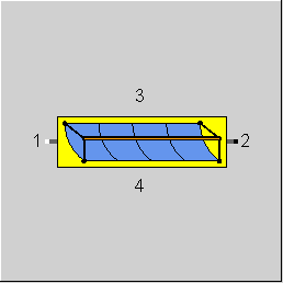
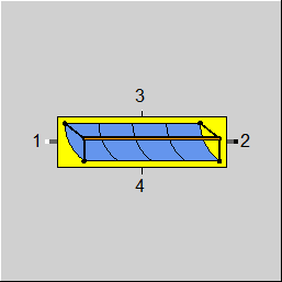
Line connections |
|
|
|
1 |
Fluid inlet |
|
|
2 |
Fluid outlet |
|
|
3 |
Limit input |
|
|
4 |
Logic output |
|
General User Input Values Physics Used Solar input: QSOLAR Characteristic Lines Displays Example
This component represents a single line-focusing solar collector which can be of parabolic trough or linear Fresnel type. For the most common systems (Eurothrough, LS-2, IST in the case of parabolic troughs, Industrial Solar (formerly Mirroxx) in the case of Fresnel), the data are already stored in the database ( Component properties window "Basic Properties"--> "Load default-values").
The underlying models calculate the energy balance from direct solar irradiation to usable heat in the heat transfer fluid. Solar and ambient data are provided by a component 117 (Sun). The component includes models with different degrees of detail which can be switched on or off by several flags. For efficiency data, the user has the possibility to define the coefficients in standard formulations, to use an adaptation function or to define data tables for interpolation.
In parallel to the thermodynamic behaviour, the component includes a model-based approach for pressure loss calculation. Empirical correlations for single and two-phase flow are available.
For controlling the focusing, a logic inlet (as previously in component 116) has been added in order to avoid a temperature transgression at the outlet. For this, the flag FFOCUS is to be set to 1 and the desired FOCUS value is to be specified as enthalpy at (logic line) pin 3. If required, this can be changed via a controller in such a way that a requested outlet state is achieved.
In addition, a logic outlet 4 for QEFF has been added.
Note on the consideration of the wind impact:
As the impact of wind speed and wind direction individually depends on the respective plant and the ambient landscape, there are no general formulae for calculating this impact. Therefore the tuning factor CORWIND for the wind impact has the default value 1, i.e. no wind impact is considered. If it is known how great the wind impact is, the corresponding tuning factor for the wind impact can be entered manually in CORWIND.
If it is even known how the wind impact depends on wind speed and wind direction, Ebsilon allows to store this dependency in a Kernel expression EWIND. For EWIND to be used, the flag FWIND has to be switched to 1 (use of EWIND).
For creating the Kernel expression, the component provides the following variables as KE_Internals:
The flag FSWIND determines whether the local values from the component or the superordinate values from the sun component are used for VWIND and AWIND.
The result of the Kernel expression EWIND must be between 0 and 1. This value is then multiplied by the specification value CORWIND and subtracted from 1 in order to obtain the efficiency for the wind impact:
ETAWIND = 1 – CORWIND * EWIND
Thus in the case of EWIND=0, there is no wind impact and
in the case of EWIND=1, the maximum wind impact exists.
The efficiency then decreases by a fraction CORWIND.
Please note that for historical reasons CORWIND is interpreted differently in the case of FWIND=0 and FWIND=1.
In the case of FWIND = 0, CORWIND is the tuning factor for the efficiency (i.e. CORWIND=1 means no correction); in the case of FWIND = 1, CORWIND is the fraction by which the efficiency is maximally decreased (i.e. CORWIND=0 means no correction).
|
COLSET |
Name of collector set load |
|
FTYPE |
Collector type Expression =0: Parabolic Trough =1: Linear Fresnel |
|
LENGTH |
Gross length of the collector module |
|
AWIDTH |
Gross aperture width of the collector module |
|
NRATIO |
Optical active portion of aperture: Ratio of active reflective area to gross collector area given by LENGTH*AWIDTH |
|
LFOCAL |
Focal length of collector (Parabolic Trough) / Height of absorber tube over mirror plane (Linear Fresnel) (used for endless calculation) |
|
DINNER |
Inner diameter of absorber tube |
|
ROWDIST |
Distance of the axis of two parallel collector rows (used for shading calculation) |
|
CDIST |
Distance between two collectors in series |
|
CAZIM |
Collector azimuth angle: Direction of the positive collector axis. Towards north=0°, positive in eastern direction |
|
CSLOP |
Collector axis slope: Angle between collector axis and horizontal plane (used for calculation of incident and transversal angle if FSPHI=2) |
|
FMODE |
Flag for calculation mode (design / off-design) Expression = 0: Global |
|
FDP12N |
Method for calculation of nominal pressure loss Expression =0: Given by parameter DP12N =1: Model based calculation |
|
DP12N |
Nominal pressure loss (this value is used if FDP12N=0) |
|
NNODEP |
Nodes for pressure loss calculation |
|
FDP12PL |
Method for calculation of part-load pressure loss Expression =0: Depending on mass flow =1: Depending on mass and volume flow =2: Constant at nominal value (calculated according to FDP12N) =3: Model based calculation =4: Adaptation function EDP12PL |
|
EDP12PL |
for FDP12PL=4 adaptation function part-load pressure drop in relation to nominal pressure drop. |
|
KS |
Equivalent sand roughness of absorber pipe inner surface (this value is used if FDP12N=1) |
|
ZETA |
Pressure loss coefficient for additional pressure losses not covered by the pressure loss model (used if FDP12N=1) |
|
FOPT0 |
Peak optical efficiency (related to the net aperture area LENGTH*AWIDTH*NRATIO at PHIINC=0) |
|
CLEANI |
Cleanliness of the mirrors as a ratio of actual reflectivity to nominal reflectivity assumed for FOPT0 (standard value is 1 indicating clean mirrors) |
|
FFOCUS |
Specification of focus state Expression =0: By specification value FOCUS |
|
FOCUS |
Focus state of the collector (0=not focused, 1=focused, linear in between) |
|
CORSHAD |
Factor to tune the result of the shading model (0= no shading, 1=based on model) |
|
FELOSS |
Method for calculation of optical end losses and end gains Expression =0: Optical end losses not considered (also end gains not considered) =1: End losses considered according to model and tuning factor CORELOS =2: End losses and end gains at inflow side of collector considered according to model and tuning factors CORELOS and COREGAI are used =3: End losses and end gains at outflow side of collector considered according to model and tuning factors CORELOS and COREGAI are used =4: End losses and end gains at both sides of collector considered according to model and tuning factors CORELOS and COREGAI are used |
|
CORELOS |
Factor to tune the optical end losses calculated from the end loss model (1=no correction of model) |
|
COREGAI |
Factor to tune the optical end gains calculated from the end gain model (1=no correction of model) |
|
FWIND |
Tuning factor for wind impact (1=no correction) Expression =0: Given by factor CORWIND (Note: Specification values SVWIND and AWIND remain grayed out, even if FSWIND switches over.) =1: Adaptation function EWIND |
|
CORWIND |
Factor to describe wind impact on optical performance Standard value = 1 (no influence) |
|
EWIND |
for FWIND=1 adaptation function wind impact: |
|
NNODE |
Number of nodes along the collector axis used for the calculation of the heat losses. The temperature difference along the collector is divided into NNODE intervals. Heat losses are calculated in the center of each section. |
|
FSPHI |
Definition of incident and transversal angle Expression =0: Given by parameters PHIINC and PHITRAN =1: Incident and transversal angle taken from calculation in superior SUN component with index ISUN =2: Incident and transversal angle calculated from collector orientation (given by parameters CAZIM and CSLOP) and sun position obtained from superior SUN component with index ISUN |
|
PHIINC |
Incident angle prescription (this value is used if FSPHI=0) |
|
PHITRAN |
Transversal angle prescription (this value is used if FSPHI=0) |
|
FSDNI |
Definition of direct normal irradiance Expression =0: Given by parameter DNI =1: Taken from superior SUN component with index ISUN |
|
DNI |
Direct normal irradiance (this value is used if FSDNI=0) |
|
FSTAMB |
Definition of ambient temperature Expression =0: Given by parameter TAMB =1: Taken from superior SUN component with index ISUN |
|
TAMB |
Ambient temperature (this value is used if FSAMB=0) |
|
FSWIND |
Definition of wind speed and wind direction (FWIND=1) Expression =0: Given by parameters VWIND and AWIND =1: Taken from superior SUN component with index ISUN (Note: FSWIND only specifies whether the wind speed and wind direction are specified individually for the solar collector |
|
VWIND |
Wind speed (>0, this value is used if FSWIND=0) |
|
AWIND |
Wind direction (from south to north=0°, positive in east direction, values in the range of 0..360°, this value is used if FSWIND=0) |
|
ISUN |
Index of reference solar data component |
Note for VWIND und AWIND: Note for VWIND and AWIND: EBSILON does not calculate the wind influence and does not use these default values unless the user
defines it himself via EWIND.
Then he can use VWIND and AWIND, including the setting in FSWIND, i.e. H. VWIND and AWIND can also be taken from component 113.
|
FIAM |
Method for calculation of incident angle correction Expression =0: Standard polynomial =1: Adaptation functions defined in EPHIINC and EPHITRAN =2: Table based values given by CIAMINC and CIAMTRAN |
|
IAMLA |
Coefficient for standard formulation (longitudinal) (A-Term) |
|
IAML0 |
Coefficient for standard formulation (longitudinal) (constant Term) |
|
IAML1 |
Coefficient for standard formulation (longitudinal) (linear Term) |
|
IAML2 |
Coefficient for standard formulation (longitudinal) ( ^2-Term) |
|
IAML3 |
Coefficient for standard formulation (longitudinal) ( ^3-Term) |
|
IAML4 |
Coefficient for standard formulation (longitudinal) ( ^4-Term) |
|
IAML5 |
Coefficient for standard formulation (longitudinal) ( ^5-Term) |
|
IAMLCOS |
Coefficient for standard formulation (longitudinal) (Cosine-Term) |
|
IAMT0 |
Coefficient for standard formulation (transversal) (constant Term) (FTYPE=1) |
|
IAMT1 |
Coefficient for standard formulation (transversal) (linear Term) (FTYPE=1) |
|
IAMT2 |
Coefficient for standard formulation (transversal) ( ^2-Term) (FTYPE=1) |
|
IAMT3 |
Coefficient for standard formulation (transversal) ( ^3-Term) (FTYPE=1) |
|
IAMT4 |
Coefficient for standard formulation (transversal) ( ^4-Term) (FTYPE=1) |
|
IAMT5 |
Coefficient for standard formulation (transversal) ( ^5-Term) (FTYPE=1) |
|
IAMTCOS |
Coefficient for standard formulation (transversal) (Cosine-Term) (FTYPE=1) |
|
EPHIINC |
for FIAM=1 adaptation function for incident angle. Result: 0...90° |
|
EPHITRAN |
for FIAM=1 and FTYPE=1 adaptation function for transversal angle. |
|
FQLOSS |
Method for heat loss calculation Expression =0: Standard polynomial =1: Adaptation function defined in EQLOSS =2: Table based values given by QLOSSA and QLOSSB |
|
QLOSSA0 |
Coefficient for standard formulation heat loss (no DNI dependency) (constant Term in dT) |
|
QLOSSA1 |
Coefficient for standard formulation heat loss (no DNI dependency) (linear Term in dT) |
|
QLOSSA2 |
Coefficient for standard formulation heat loss (no DNI dependency) (^2 Term in dT) |
|
QLOSSA3 |
Coefficient for standard formulation heat loss (no DNI dependency) (^3 Term in dT) |
|
QLOSSA4 |
Coefficient for standard formulation heat loss (no DNI dependency) (^4 Term in dT) |
|
QLOSSB0 |
Coefficient for standard formulation heat loss (DNI dependency) (const. Term in dT) |
|
QLOSSB1 |
Coefficient for standard formulation heat loss (DNI dependency) (lin. Term in dT) |
|
QLOSSB2 |
Coefficient for standard formulation heat loss (DNI dependency) (^2 Term in dT) |
|
QLOSSC1 |
Coefficient for standard formulation heat loss (no DNI dependency) (lin. Term in T) |
|
QLOSSC2 |
Coefficient for standard formulation heat loss (no DNI dependency) (^2 Term in T) |
|
QLOSSC3 |
Coefficient for standard formulation heat loss (no DNI dependency) (^3 Term in T) |
|
QLOSSC4 |
Coefficient for standard formulation heat loss (no DNI dependency) (^4 Term in T) |
|
QLOSSD1 |
Coefficient for standard formulation heat loss (DNI dependency) (lin. Term in T) |
|
QLOSSD2 |
Coefficient for standard formulation heat loss (DNI dependency) (^2 Term in T) |
|
EQLOSS |
for FQLOSS=1 adaptation function for receiver heat losses. Result: [W/m] |
|
M1N |
Mass flow (nominal) |
|
VREFN |
Specific volume at reference point (nominal) |
The parameters marked in blue are reference quantities for the off-design mode. The actual off-design values refer to these quantities in the equations used.
Generally, all inputs that are visible are required. But, often default values are provided.
For more information on colour of the input fields and their descriptions see Edit Component\Specification values
For more information on design vs. off-design and nominal values see General\Accept Nominal values
|
RDNI |
Direct normal irradiance used for calculation |
|
RSHEIGHT |
Sun height angle used for calculation |
|
RSAZIM |
Sun azimuth angle used for calculation |
|
RPHIINC |
Incident angle used for calculation |
|
RPHITRAN |
Transversal angle used for calculation |
|
ETACOLL |
Collector efficiency QEFF / (RDNI*ANET) |
|
RFOCUS |
Value used for FOCUS |
|
QSOLAR |
Solar heat input |
|
QLOSS |
Heat losses collector |
|
QEFF |
Heat absorbed by fluid |
|
QLSOLAR |
Length specific solar heat input |
|
QLLOSS |
Length specific heat losses |
|
QLEFF |
Length specific effective heat |
|
QASOLAR |
Area specific solar heat input QSOLAR/ANET |
|
QALOSS |
Area specific heat losses QLOSS/ANET |
|
QAEFF |
Area specific effective heat QEFF/ANET |
|
ANET |
Net aperture area |
|
TAVER |
Average collector temperature 0.5*(T1+T2) |
|
KIA |
Incident angle modifier |
|
KIAINC |
Incident angle modifier (longitudinal part) |
|
KIATRAN |
Incident angle modifier (transversal part) |
|
ETASHAD |
Shading efficiency |
|
ETAENDL |
Endless efficiency |
|
ETASPILL |
Spillage efficiency |
|
DP12 |
Pressure loss over collector |
|
RVWIND |
Wind speed used in calculation |
|
RAWIND |
Wind direction used in calculation |
|
RTAMB |
Ambient temperature used in calculation |
General heat balance
The heat input into the fluid flow is given by
M1*(H2-H1) = QEFF .
This equation is used for both parabolic trough and Linear Fresnel collectors. The effective heat input QEFF depends on the solar heat input QSOLAR and the thermal losses QLOSS.
QEFF = QSOLAR - QLOSS
The solar input QSOLAR is determined by the equation
QSOLAR = DNI * ANET * FOPT_0 * KIA * FOCUS * ETASHAD * ETAENDL * ETASPILL * ETA_CLEAN
with the terms:
DNI Direct normal irradiance in W/m**2
ANET Net aperture area ANET=LENGTH*AWIDTH*NRATIO
FOPT_0 Peak optical efficiency (parameter FOPT0)
KIA Incident angle correction (cosine losses already included)
FOCUS Focus state of the collector
ETASHAD Factor to include shading losses
ETAENDL Factor to correct end loss effects determined from model
ETASPILL Factor to include optical losses due to wind impact
ETA_CLEAN Factor to correct for actual mirror cleanliness ETA_CLEAN=CLEANI
The heat losses of the collector to the surrounding are calculated based on the length-specific heat loss QLOSS by
QLOSS = qloss * LENGTH
The applied methods for the calculation of the terms are provided in the following section.
The performance of the collector depends on the product
FOPT0 * LENGTH * AWIDTH * NRATIO .
Since performance data found in literature do not have a unique structure please make sure that FOPT0 is always used together with the corresponding reference area. This might be the gross area as given by LENGTH*AWIDTH or the net area which is reduced by factor NRATIO. If the gross area is reported as the reference, NRATIO should be equal to 1 to come to correct results.
For Linear Fresnel systems AWIDTH is considered as the width of the collector system. Due to the facetted structure, NRATIO is used to define the net aperture area. It is in the choice of the manufacturer if the net aperture area is defined as the area if all facettes are looking to the zenith or the one of the projected area at perpendicular irradiation. For correct results the aperture area definition should be consistent with the peak optical efficiency value and the incident angle correction values KIA.
For linear Fresnel systems the peak optical efficiency might not be reached at perpendicular irradiance due to the specific optics of these systems. Two options for defining the parameters are open to the user:
The peak optical efficiency FOPT0 describes the optical efficiency of the collector under the assumptions
Deviations from this ideal reference point are described by a number of factors that reduce the available heat. These are described in the following.
Incident angle correction: KIA
At non-perpendicular incident of the sun additional losses due to shading of collector structure elements, a longer optical path of the reflected sun rays and angle-dependent optical properties of mirrors and absorber tube occur. These optical effects are summarized in the incident angle correction KIA. Note that this factor already includes the cosine losses of the parabolic trough collector in order to allow the same methodology as for linear Fresnel systems.
KIA = KIAINC(RPHIINC) for parabolic trough systems,
KIA = KIAINC(RPHIINC) * KIATRAN(RPHITRAN) for linear Fresnel systems
(with RPHITRAN=abs(PHITRAN)) .
The user has three options to specify the relations between the angles RPHIINC, RPHITRAN and KIAINC and KIATRAN which are chosen by flag FSPHI.
KIAINC = ( 1-IAMLA+IAMLA*cos(RPHIINC) ) * (IAMLCOS*cos(RPHIINC) + IAMLO + IAML1*RPHIINC + IAML2*RPHIINC**2 + IAML3*RPHIINC**3 + IAML4*RPHIINC**4 + IAML5*RPHIINC**5 )
The structure of this function is chosen to be able to represent common formulations from literature. The terms in the first bracket are necessary if a polynomial-based relation for the incident angle correction has to be represented which does not already include the cosine of the incident angle.
For the Linear Fresnel system the correlations
KIAINC = IAMLO + IAML1*RPHIINC + IAML2*RPHIINC**2 + IAML3*RPHIINC**3 + IAML4*RPHIINC**4 + IAML5*RPHIINC**5
KIATRAN = IAMTO + IAMT1*RPHITRAN + IAMT2*RPHITRAN**2 + IAMT3*RPHITRAN**3 + IAMT4*RPHITRAN**4 + IAMT5*RPHITRAN**5
are used. In all cases the results of the functions are limited to a minimum value of 0. When using the adaptation function or table based method always check if the units (deg or rad) of RPHIINC, RPHITRAN fit to the values you specify.
If the sun is near the horizon, parallel collector rows shade each other. This effect is considered by means of the term ETASHAD which is calculated based on geometric relation in dependence of the track angle (=transversal angle) of parabolic trough systems.
ETASHAD=1 - min(1, CORSHAD * max( 0,1- ROWDIST * cos(RPHITRAN) / AWIDTH ) )
The term min(...) describes the reduction of available energy as a fraction of the energy available if no shading occurs. If the sun is high above the horizon this term equals to 0 and the ETASHAD is 1. The user has the possibility to tune the model based shading effect by a tuning factor CORSHAD.
At incident angles <>0 some fraction of the reflected sun beams at the ends of the collector do not hit the absorber tube. This effect is called optical end loss and is a function of the incident angle RPHIINC. If the next collector is arranged in the same axis the lost sun beams of one collector can hit the absorber tube of the next collector. A fraction of the lost heat can be therefore be regained. This effect is called optical end gain. Since a collector can have a corresponding neighbour collector at one side or at both sides, the effective end gains depend on the position of the collector in the field. The user has the possibility to specify at which end of the collector end gains can be obtained. End gains are always less than the end losses. The flag FELOSS defines in which way the end effects are handled:
The end loss effects ETA_ELOS are calculated based on the equation
ETA_ELOS =1
- CORELOS * min(1, kel * LFOCAL/LENGTH * tan(RPHIINC) )
+ COREGAI * max( 0, keg*min(1, kel * LFOCAL/LENGTH * tan(RPHIINC) ) - CDIST/LENGTH )
where the term with CORELOS represents the end losses and the term with COREGAI represents the end gains. The parameters CORELOS and COREGAI are tuning factors with a default value of 1 that correct the calculated effects by a factor. The values kel and keg are used to include the user's choice in flag FELOSS:
For the calculation based on FELOSS=2, 3 the sun position (azimuth angle SAZIM) is required to determine the sun position relative to the collector. The sun position has to be provided by the sun model with index ISUN. For the other options the sun position is not required to calculate the end losses.
Under wind loads the collector structure is deformed which reduces the optical efficiency. This effect is represented by the factor ETASPILL. There is no model or standard formulation for the spillage effect included, as this data on this effect are sparse. The user has two possibilities:
The actual cleanliness of the mirrors relative to the ideally clean state can be specified by parameter CLEANI so that ETA_CLEAN=CLEANI.
Due to a temperature difference between the heat transfer fluid and the ambient air, heat losses occur in the collector. Heat losses are assumed to only depend on the temperature difference. The user has three options to specify the heat loss qloss per unit length of the collector:
The predefined function is given as
where T-Tamb is the temperature difference between fluid and ambient air and hopt is defined as:
hopt= KIA * FOCUS * ETASHAD * ETAENDL * ETASPILL * ETA_CLEAN .
The formulation of the predefined function is chosen in a way that common formulations from literature can be represented. The terms with QLOSSAx model a simple heat loss term that only depends on the fluid temperature which is a simplifying assumption. In effect the heat loss is dependent on the temperature on the outside of the absorber tube. This temperature is thus dependent on the actual radial heat flow which goes in a first approximation linear with the effective irradiance RDNI*hopt. The terms with QLOSSBx are added to model this impact. The polynomial for calculating the heat losses has been expanded by such fractions that directly depend on the temperature (QLOSSC1 to QLOSSC4, QLOSSD1, QLOSSD2).
|
QLOSSA0 |
W / m |
|
QLOSSA1 |
W / (m K) |
|
QLOSSA2 |
W / (m K**2) |
|
QLOSSA3 |
W / (m K**3) |
|
QLOSSA4 |
W / (m K**4) |
|
QLOSSB0 |
m |
|
QLOSSB1 |
m / K |
|
QLOSSB2 |
m / K**2 |
|
QLOSSC1 |
W / (m °C) |
|
QLOSSC2 |
W / (m °C**2) |
|
QLOSSC3 |
W / (m °C**3) |
|
QLOSSC4 |
W / (m °C**4) |
|
QLOSSD1 |
m / °C |
|
QLOSSD2 |
m / °C**2 |
With the resulting formula two commonly used formulations can be represented. This is illustrated in the following:
The correlation for collector efficiency suggested early by Sandia National Laboratories reads
eta[%] = KIA * (73.3-0.007276*dT) - 0.496*dT / DNI - 0.0691 * dT**2 / DNI .
In order to obtain the corresponding values for the EBSILON®Professional formulation the %-formulation and the sign have to be considered. Further the SANDIA formulation is based on the aperture area whereas the formulation here is length-specific. With an aperture width for the above given LS-2 collector, the parameters are obtained as:
|
QLOSSA0, QLOSSA3, QLOSSA4 = 0 |
|
QLOSSA1 = 0.496 W%/(m**2 K) * 5.0 m / 100% = 0.0248 W/ (m K) |
|
QLOSSA2 = 0.0691 W%/(m**2 K**2) * 5.0 m / 100% = 0.003455 W/ (m K**2) |
|
QLOSSB0, QLOSSB2 = 0 |
|
QLOSSB1 = 0.007276 %/K * 5.0 m / 100% = 0.0003638 |
The correlation for the heat losses of a Eurotrough collector have been published as
Qloss[W/m**2] = 0.00047 W/(m**2 K**) * dT**2 .
This area-specific heat loss can simply be transformed into the length-specific heat loss formulation with the net aperture width of 5.45 m (values were obtained based on net area):
|
QLOSSA0, QLOSSA1, QLOSSA3, QLOSSA4 = 0 |
|
QLOSSA2 = 0.00047 W/(m**2 K**) * 5.45 m = 0.0025615 W/ (m K**2) |
|
QLOSSB0, QLOSSB1, QLOSSB2 = 0 |
The heat loss the user can specify the number of sections to be taken as a basis in the calculation (specification value NNODE). This calculation by sections is also possible for the pressure drop, too (specification value NNODEP).
The user has the following options for the calculation of the nominal pressure loss:
The user has the following options for the calculation of the part-load pressure loss:
To cover single and two-phase flow with one consistent model the two-phase pressure loss model by Friedel (VDI-Wärmeatlas) is used. This model is described in the following. The calculation of pressure drop coefficients is based on single phase Reynolds numbers RE_L and RE_G
RE_L = MFLUX * DINNER / ETA_L
RE_G = MFLUX * DINNER / ETA_G
with the mass flow density MFLUX=M1/(pi/4*DINNER**2) and the dynamic viscosities of liquid (ETA_L) and gas (ETA_G). For two-phase flow, these Reynolds numbers are calculated as if each phase flows alone in the pipe. The single phase pressure loss coefficients are calculated as
ZETA_L=( 0.86859 * ln( RE_L / (1.964 * ln(RE_L) - 3.8215) ) )**(-2) for RE_L > 1055
ZETA_L=64 / RE_L for RE_L < 1055
ZETA_G=( 0.86859 * ln( RE_G / (1.964 * ln(RE_G) - 3.8215) ) )**(-2) for RE_G > 1055
ZETA_G=64 / RE_G for RE_G < 1055 .
The term
DP_L=ZETA_L * MFLUX**2 / (2*DINNER*RHO_L)
describes the specific pressure loss (Pa/m), as if the whole mass were be present as liquid. A two-phase multiplier R is used to consider the impact of the gas phase
DP_S = DP_L * R .
For calculation of R the Weber number
WE_L = MFLUX**2 * DINNER / RHO_L / SIGMA.
and the Froude number
FR_L = MFLUX**2 / ( 9.81 * DINNER * RHO_L**2 )
of the liquid phase are required. With these numbers the terms
A = (1-X)**2 + X**2 * (RHO_L * ZETA_G / RHO_G / ZETA_L)
VV = (RHO_L/RHO_G)**0.8 * (ETA_G/ETA_L)**0.22 * (1-ETA_G/ETA_L)**0.89 * FR_L**(-0.047) * WE_L**(-0.0334)
XX = 3.43 * X**0.685 * (1-X)**0.24
R = A + XX * VV
are calculated where X is the gaseous fraction of the flow (kg/s of gas per kg/s of total flow) and RHO and ETA are the density and the dynamic viscosity of gas and liquid.
This model can be used in the whole range from single phase liquid flow over two-phase flow to single phase gas flow. This model does not consider pipe roughness.
Since standard models for two-phase pressure drops in rough pipes are not available the following assumption is made. In the single phase regions the pressure loss in rough pipes is calculated by the correlation
ZETA_LR = 0.25 * ( log10( KS /(3.7*DINNER) + 5.74 /RE_L**0.9 ) )**(-2)
ZETA_GR = 0.25 * ( log10( KS /(3.7*DINNER) + 5.74 /RE_G**0.9 ) )**(-2)
of Swamee and Jain (1976) which approximates the well known implicit equation by von Karman and Nikuaradse. The corresponding pressure losses are
DP_LR = ZETA_LR * MFLUX**2 / (2*DINNER*RHO_L)
DP_GR = ZETA_GR * MFLUX**2 / (2*DINNER*RHO_G) .
Due to a lack of reliable models the pressure drop in rough pipes in the two-phase region is approximated as
DP_R = DP_LR + (DP_GR-DP_LR) * X
The final pressure drop is defined as the maximum of the smooth pipe pressure drop DP_S and the rough pipe pressure drop DP_R as
DP = max ( DP_S, DP_R) .
This approach has the advantage that the single phase pressure drops are represented very well. A common model for two-phase pressure drop is also available. With the approach defined here the pressure drop is continuous at the boundaries X=0 and X=1.
Fluid properties (enthalpy, pressure, steam fraction, ...) for pressure loss calculation are taken from the center of the collector.
In addition to the pressure loss calculation for the pipe flow the user may enter a pressure loss coefficient ZETA to generate the additional pressure drop
DPZETA = ZETA * RHO * ( MFLUX / RHO )**2
In case of two-phase flow the mass averaged mixture density RHO is used. The density is evaluated in the center of the collector (H1+H2)/2 and (P1+P2)/2.
CIAMINC: Incident Angle Modifier (Longitudinal)
Correction Factor = f(PHIINC)
CIAMTRAN: Incident Angle Modifier (Transverse)
Correction Factor = f(PHITRAN)
CQLOSSA: Heat Loss (dT)
Heat Loss = f(dT)
CQLOSSB: Heat Loss (dT) / DNI
Heat Loss = f(dT) / DNI
 |
Display Option 1 |
Click here >> Component 113 Demo << to load an example.