Component 106: ENEXSA Gas Turbine (OEM GT)

In This Topic

Component 106: ENEXSA Gas Turbine (OEM GT)

Specifications

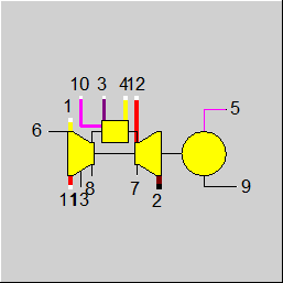
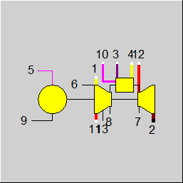
Line connections
1	Air intake
2	Exhaust gas outlet
3	Fuel inlet
4	Injection water/steam inlet
5	Generator power
6	Logic port for ambient pressure
7	Logic port for auxiliary losses
8	Logic port for cooling duty (rejected from compressor intercooler)
9	Measured power/load (Logic port for load control)
10	Fuel #2 inlet
11	Water/steam input (optional) for modelling increased performance and NOx reduction
12	Water/steam input (optional) for modelling increased performance and NOx reduction
13	Additional logic port for cooling duty

General User Input Values Characteristic Lines Physics Used Results Displays Example

General

Component 106 simulates the characteristics of a gas turbine utilizing vendor information in form of correction curves. Based on a data set (the so-called Rating) under specified reference conditions (e.g. ISO conditions) the following parameters are determined by linear interpolation between characteristic lines:

net output (power at generator terminals)
heat rate
exhaust gas flow
exhaust gas temperature
cooling duty (of gas turbine compressor intercooler, if applicable), and
water- or steam injection flow (to combustion chamber, if applicable).

The deviation between the rating under reference conditions and the current operating point is calculated as a function of the following parameters:

compressor inlet temperature
ambient pressure , defined on logic line no. 6
inlet pressure drop between ambient and compressor inlet
outlet pressure drop between turbine exit and ambient
humidity at compressor inlet
fuel lower heating value
water- or steam injection flow
grid frequency
maximal volume percentage of hydrogen and
load.

These parameters have to be specified or have to be implicitly available through connected lines. The component has several logic ports at which the following parameters can be specified:

on logic line no. 6: ambient pressure or geo-potential height
on logic line no. 7: auxiliary or other losses
on logic line no. 9: the required gas turbine net power output or load fraction.

The logic line at port 8 allows for linking the cooling duty of the gas turbine intercooler with other modules in the cycle calculation. If a gas turbine data set contains curves for cooling duty and port 8 is not connected, EBSILON will issue an error message, because in this case the heat recoverable from the intercooler would not be considered in the overall energy balance.

For the correction factors and the correction offsets, respectively, Kernel expressions can be used.

Note : The setting in the model options (Formulation gas table)

FDBR (ideal gas) for all materials excepting H2O
VDI 4670 (ideal gas, LibIdGas) for N2, O2, Ne, Ar, CO, CO2, SO2, H2Og, other FDBR
LibHuGas (real gas) für N2, O2, Ne, Ar, CO, CO2, SO2, H2Og, other FDBR
NASA (ideal gas)

is considered.

This may slightly change the results. Up to Release 11, this component internally always used the FDBR substance data for air, fuel and exhaust gas.

Specification of voltage, frequency and type of current in the component:

It is possible to specify voltage (VOLT), frequency (FREQ) and current type (NPHAS) as the default value in the component.

The flags FVOLT and FFREQ are used to set whether the specification is to be made by the new specification values VOLT and FREQ respectively (0) or externally as a measured values on the electrical line (-1).

User Input Values

GTCSET	Gas Turbine Curve Set (selected in FCURVESET)
CSET	Curve Set Description (from Library)
FLOAD	Load mode =0: Base Load =1: Desired Power (absolute) =2: Part-load Fraction (fraction of base load power under current conditions) =3: Set Operating Point (direct input of performance data) =4: Set Operating Point, accept fuel flow (e.g. for calculation of fuel flow from pressure drop across an orifice) =5: Bypass =6: Set Operating Point Externally (Data Reconciliation)
FCURVESET	Active Curve Set (selectable from drop-down list of data sets currently loaded into the component)
FFUELPRT	Fuel Port =0: Automatic, Port 3 preferred (connected fuel port will be used; if both are connected, port 3 will be used) =1: Port 3 =2: Port 10
FLOADTG	Target Values for Power/Load = 0: Use Internal Target Values (direct input of Q or LOAD) = 1: Use Port 9 enthalpy for Power/Load
Q	Power (at generator terminals)
HR	Heat Rate
M2	Exhaust Flow
T2	Exhaust Temperature
QCOOL	Cooling Duty - logic line has to be connected to port 8
QCOOL2	Additional Cooling Duty - logic line has to be connected to port 13
LOAD	Part-load Fraction
LOADMIN	Minimal Part-load Fraction (relative to base load under current conditions)
LOADMAX	Maximal Part-load Fraction (relative to base load under current conditions)
QMAX	Maximal Power output (absolute, e.g. in case of limitation by the generator or transformer)
FEBD	Energy Balance Difference Mode = 0: Calculate EBD = (Q_in - Q_out)/Q_in = 1: Set EBD, Vary Heat Rate = 2: Set EBD, Vary Exhaust Flow = 3: Set EBD, Vary Exhaust Temperature = 4: Set EBD, Vary Power = 5: Set EBD, Vary Losses = 6: Set EBD, Vary Cooling duty
FEBDMODE	Energy Balance Difference calculation mode =0: Definition specification value =1: Adaption function
EBD	Energy Balance Difference (defined as (Q_in - Q_out)/Q_in)
EEBD	Energy Balance Difference function
FQLATG	Target Values for Auxiliary Losses = 0: Use Internal Target Values (direct input of QLOSSAU) = 1: Use Port 8 enthalpy for Auxiliary Losses
QLOSSAUX	Auxiliary Losses (auxiliaries, radiation and other losses)
ETAG	Generator Efficiency
FGENF	Flag specification generator frequency =0: Defined by generator frequency from specification value GENF =1: Set externally
GENF	Generator frequency
FVOLT	Flag for flag method for specification of voltage = 0: Defined by specification value VOLT =1: Set externally
VOLT	Voltage (on electric lines)
NPHAS	Type of current =0: Set externally =1: One-phase alternating current =3: Three-phase alternating current
FCMODE	Correction values calculation mode =0: Definition specification value =1: Adaptation function
CFQ	Power Correction Factor (in addition to correction curves)
ECFQ	Adaption Function for Power Correction Factor
CFHR	Heat Rate Correction Factor (in addition to correction curves)
ECFHR	Adaption Function for Heat Rate Correction Factor function evalexpr:REAL; begin evalexpr:=1.0; end;
CFM2	Exhaust Flow Factor (in addition to correction curves)
ECFM2	Adaption Function for Exhaust Flow Correction Factor function evalexpr:REAL; begin evalexpr:=1.0; end;
COT2	Exhaust Temperature Correction Offset (in addition to correction curves)
ECOT2	Adaption Function for Exhaust Temperature Correction Offset function evalexpr:REAL; begin evalexpr:=0.0; end;
CFCOOLING	Cooling Duty Correction Factor (in addition to correction curves)
ECFCOOLING	Cooling Duty correction Factor function function evalexpr:REAL; begin evalexpr:=1.0; end;
CFM4	Injection Flow Correction Factor (in addition to correction curves)
ECFM4	Adaption Function for Injection flow correction Factor function evalexpr:REAL; begin evalexpr:=1.0; end;
FO2REF	Reference O2 Mode = 1: Use Internal O2 Reference = 2: Use Global O2 Reference (from Model Options/Calculation/O2-Reference Concentration)
O2REFCON	Reference O2 Concentration (Dry)
FCON	Specification of COCON/NOXCON (base of fractions) = 0: Volume Fraction = 1: Mass Fraction
COCON	Concentration of CO in Dry Exhaust Gas @ Ref O2 (COCON)
NOXCON	Concentration of NOx in Dry Exhaust Gas @ Ref O2 (NOXCON)
NOXSPLIT	NO-Split (NO/(NO+NO2) (Volume Fraction))

Generally, all inputs that are visible are required. But, often default values are provided.

For more information on colour of the input fields and their descriptions see Edit Component\Specification values

For more information on design vs. off-design and nominal values see General\Accept Nominal values

Characteristic Lines

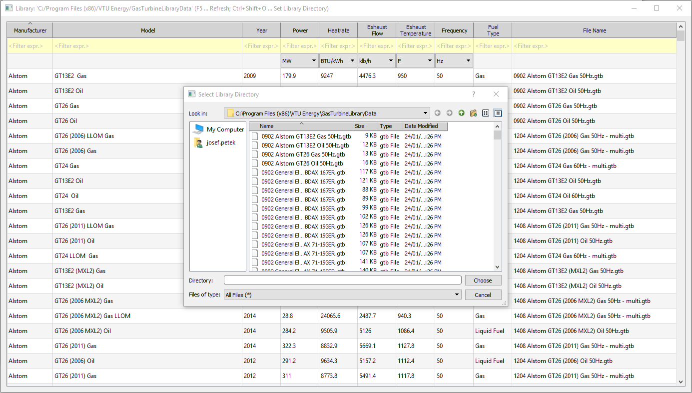
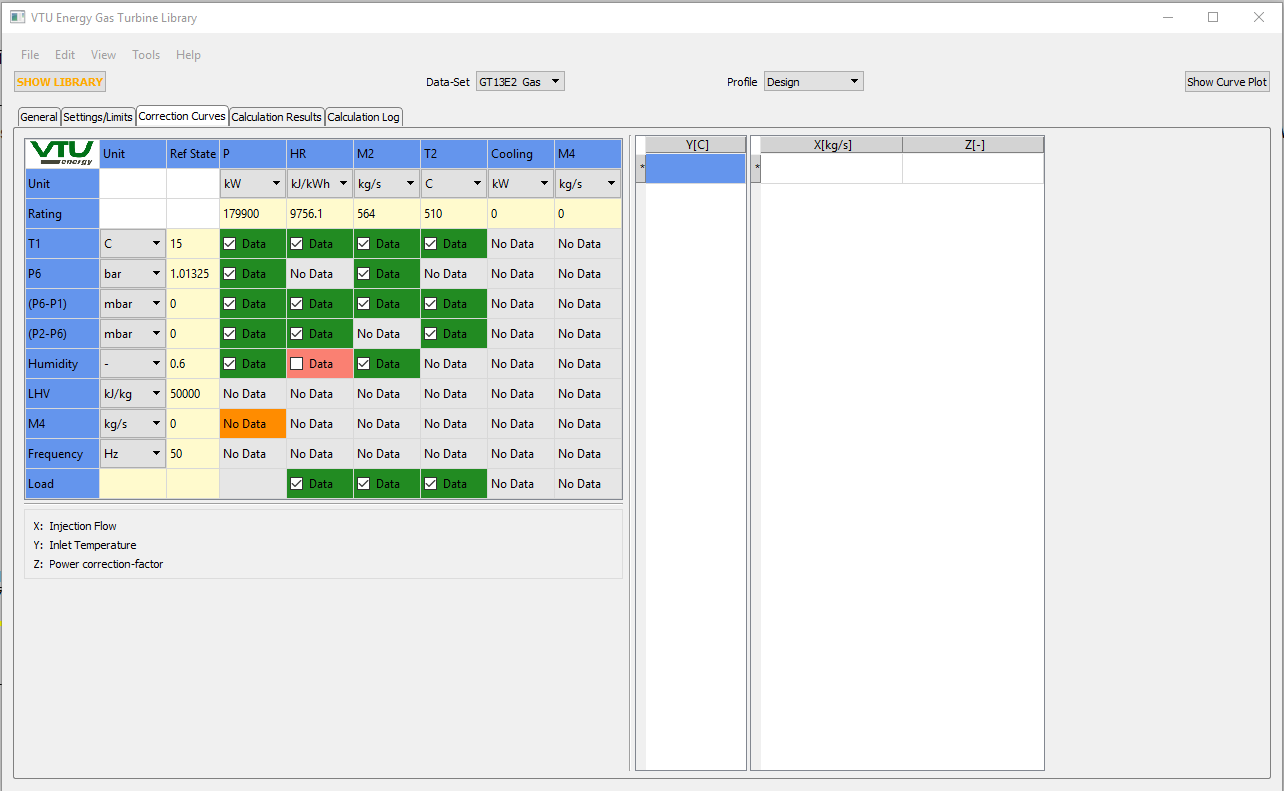
The characteristic lines for the OEM GT can be selected and edited in the Gas Turbine Library which is licensed separately by ENEXSA Energy GmbH, Austria. The entry point to the library is located in the tab ’Library’ of the OEM GT module. The picture below shows the main screen of the ENEXSA Gas Turbine Library as it will be shown upon first start-up.

Selecting the Library Location

On the left-hand side of the menu bar the command ’SHOW LIBRARY’ will activate a window showing the content of the current library directory (default path 'C:\Program Files (x86)\ENEXSA Energy\Gas Turbine Library'). Pressing the key combination "Ctrl+Shift+O" opens the Select Library Directory window that allows for selecting an alternate path to a location of the correction curve data sets which are stored in a proprietary file format with the extension *.gtb. An unlimited number of other locations can be used to create back-up copies of the library, to collect project specific data, or to save new or modified data sets.

After the path has been entered or selected in the browser window, all data sets present in the current library location will be displayed in a list view of the Library. If new files have been added to the directory, you can press function key F5 to refresh the content of the list.

Searching the Library

The top row of the table contains the column headers. Clicking on a header field will sort the content of the respective column in ascending and descending order, respectively. The second row of the table contains a filter tool that allows for searching expressions in the text of a field or for defining the desired value range with a specific syntax ('lower limit;upper limit', '> lower limit', or '< upper limit'). Where applicable, the third row of the table contains drop-down lists for the respective units of measure of the property.

Selecting the Correction Curve Set

By double-clicking in any field of a row, the respective data set will be loaded, and the following dialog will be displayed:

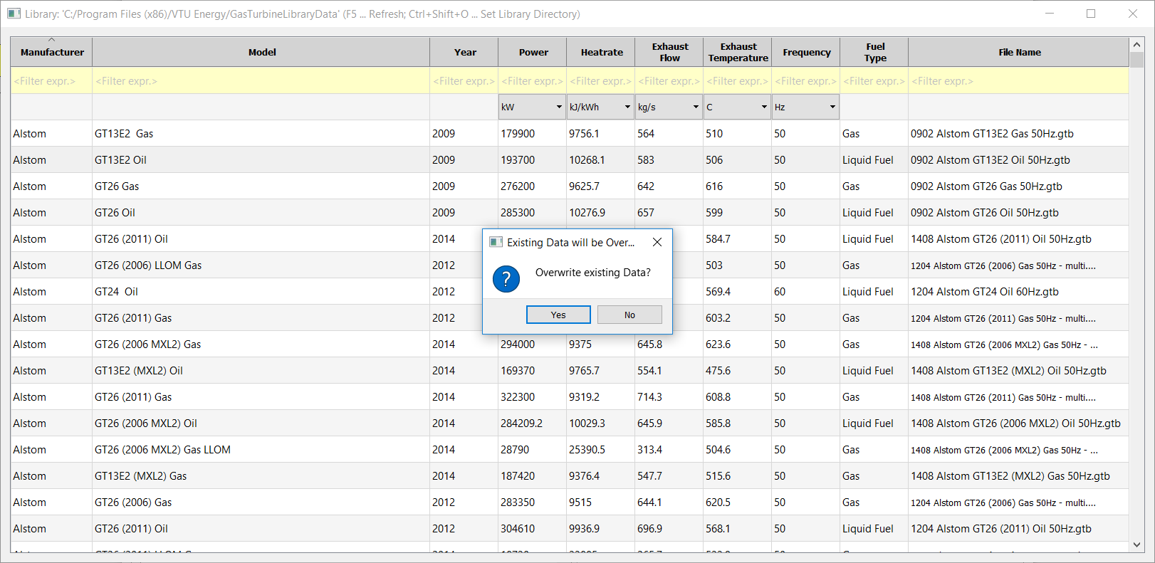
In addition to simply overwriting the current data set, the File menu of the Gas Turbine Library allows for loading several data sets into component 106:

Select 'Insert Data Set from File', if you want to insert an additional data set before the current active data set. The new data set will be active.

Select 'Append Data Set from File', if you want to add the data set after the last set in the list of data sets already loaded into the component. The new data set will not be active and needs to be selected from the drop-down list of available curve sets in the menu bar.

The drop-down list of the loaded gas turbine data sets shows the names of the respective curve sets which can be selected in the parameter FCURVESET in the specification values of component 106. The set that is currently selected will be used in the calculation, but the parameter FCURVESET may also be set in a script or through the Excel interface utilizing the integer number assigned to each data set. This feature enables you to switch between different curve sets without having to edit the model. As shown in the screen shot above, you can for instance load curve sets for operation with natural gas and distillate oil into a model and simulate the operation with both fuels in one go. Another application of this feature is for instance the special low load operating point of the Alstom GT26 gas turbine which is modelled in the ENEXSA Gas Turbine Library in a separate curve set.

When a curve set is activated, all data and correction curves present in this data set will be displayed. All data of a data set can be edited by the user. In order to include the current data in the heat balance calculation of EBSILON you have to close the gas turbine library and select ’OK’ when closing the OEM GT component in EBSILON. By this command all data will be stored in the EBSILON model, but the original data set will not be changed. The model can now be executed, even if the original data set differs from the data currently saved to the model, or even if the original data file is not present any longer (e.g. if the model has been exchanged without including the library file).

In the gas turbine library one separate file with the file extension *gtb exists for every gas turbine data set. Via the menu item ’File' à 'Load/Replace from File’ a data set can be loaded separately, and by choosing the menu item ’File' à 'Save Current Data Set to File’ the current data set can be saved to a file which is useful when adapting original data. With the command 'Save Data Set Group to File' all data sets that are currently loaded in component 106 can be saved to a single file.

The Correction Procedure

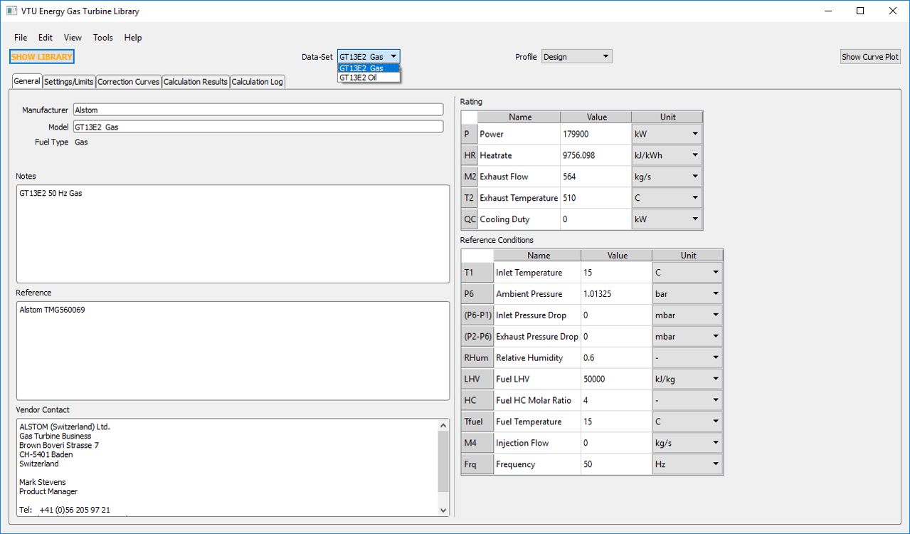
Each data set contains data for the gas turbine model, contact information of the vendor, the rating and the respective reference conditions, and up to 53 correction curves for the values of

Power (Q)
Heat Rate (HR)
Exhaust Flow (M2)
Exhaust Temperature (T2)
Cooling Duty (if applicable), and
Water or Steam Injection Flow (M4, if applicable).

as functions of the parameters

Compressor Inlet Temperature (T1)
Ambient Pressure (P6),
Inlet pressure Drop (P6-P1)
Outlet Pressure Drop (P2-P6)
Humidity
Lower Heating Value (LHV)
Water/Steam Injection Flow (M4)
Grid Frequency, and
Part-load.

Settings/Limits

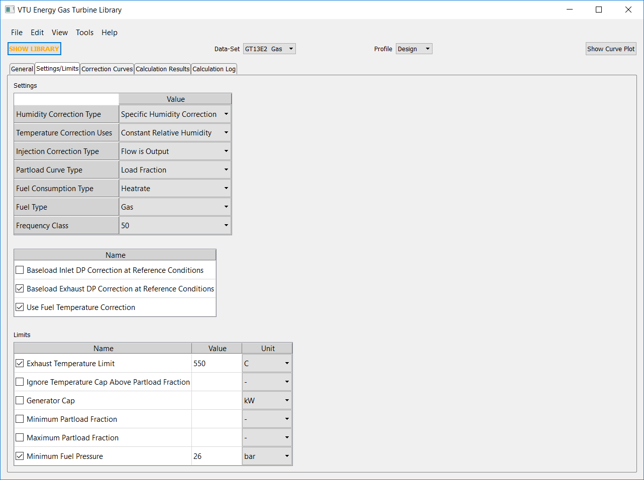
Since several of the above parameters are specified differently by the original equipment manufacturers, the following parameters are specified for each gas turbine curve set in the tab 'Settings/Limits' of the Library:

Definition	Options
Humidity Correction Type	- Relative Humidity (% of saturation) - Specific Humidity (kg / kg wet) - Humidity Ratio
Temperature Correction Type	- Constant Relative Humidity - Constant Specific Humidity
Injection Correction Type	- Injection/Fuel Flow Ratio - Injection Flow (absolute) - Injection Flow Is Output (i.e. calculated from curve set, determines M4)
Part-load Curve Type	- Power (absolute) - Load Fraction (relative to base load under current conditions) - Reference Load Fraction (relative to rating output)
Fuel Consumption Type	- Heat Rate - Heat Consumption (absolute)
Fuel Type	- Unknown - Gas - Liquid Fuel
Frequency Class
Maximum allowed H2 volume fraction in the fuel	- Volume pecventage (Mole fraction)

For existing data sets these settings must not be changed, except for the setting for Part-load Curve Type and Fuel Consumption Type. For these two settings, conversion procedures exist which transfer the data to the respective new format. If you create your own data set based on vendor data, you have to ensure that your input is in concurrence with the definition of all of the above settings with those of the respective vendor.

In addition, the Settings/Limits tab includes the following the following limits or options that can be activated by the respective check boxes:

the option Base Load Inlet DP Correction at Reference Conditions which activates an accurate mode of calculating the correction factor for inlet pressure drop which accounts for the change in inlet flow and temperature at off-design/part-load conditions and the associated pressure losses in the intake system.
the option Base Load Exhaust DP Correction at Reference Conditions which activates an accurate mode of calculating the correction factor for exhaust pressure drop which accounts for the change in exhaust flow and temperature at off-design/part-load conditions and the associated pressure losses in the exit duct/HRSG, and
the option Use Fuel Temperature Correction which activates the correction of the heat rate curve due to the change in sensible heat of the fuel entering the gas turbine, if the fuel has a different temperature than stated in the reference conditions.
an Exhaust Temperature Limit, which - most appropriately in combination with the Energy Balance Difference Mode to vary the heat rate - can be used to reflect the characteristics of certain control systems with respect to such a limit.
Since some gas turbine models allow to exceed the exhaust temperature limit at and close to base load when operating at higher ambient temperature, the respective part load fraction above which this limit shall be ignored can be specified in the input titled "Ignore Temperature Cap Above Load Fraction".
a Generator Cap which defines the maximum electrical power output by the generator. In the simulation - similar to the actual control scheme of the gas turbine - the maximum output of the gas turbine will be capped with this value, i.e. the gas turbine will be controlled to the part-load level which produces the specified maximum generator output.
the Minimum Part-load Fraction which defines the lower operating limit of the gas turbine, as for instance required by the OEM for achievement of certain NOx emission levels. If the value for the gas turbine part-load level is below this limit - be it through user input or due to an internal control logic of the model - an error message will be generated, even if the mass and energy balances are solved successfully.
the Maximum Part-load Fraction which defines the upper operating limit of the gas turbine. Some gas turbine vendors allow for temporary 'peaking operation' with elevated combustion temperature for maximizing the power output. If activated, this optional input will override the specification value LOADMAX in component 106. If the value for the gas turbine part-load level is above this limit - be it through user input or due to an internal control logic of the model - an error message will be generated, even if the mass and energy balances are solved successfully.
the Minimum Fuel Pressure which will be checked in the calculation, and in case this limit is violated, a warning will be generated.

The procedure for correction due to pressure drop at part-load conditions in the above points 1 and 2 includes the following steps:

Correction Curves

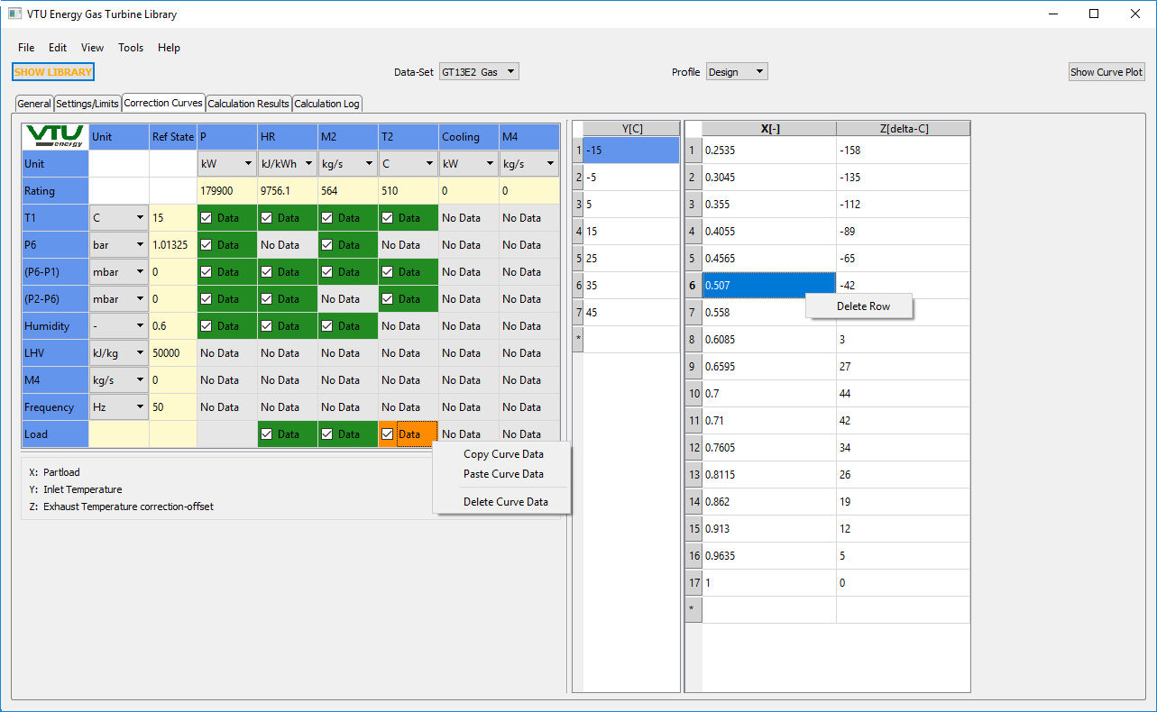
As can be seen from the picture below, the correction curves are first displayed in the tab ’Correction Curves’ in an overview matrix in which the availability of data is indicated by dark-green colouring of the respective field. Optionally, the user can set individual corrections to the status ’Disabled’ (colour code red) by unchecking the respective check box. If a data set does not contain a correction for a specific parameter, the respective field will be marked with the text ’No Data’. The current selected correction curve field is highlighted with orange colour, and if no data are present, the right-hand side Y-X-Z tables remain empty. The types of the parameters X,Y, and Z are displayed on the left-hand side below the matrix of correction curves.

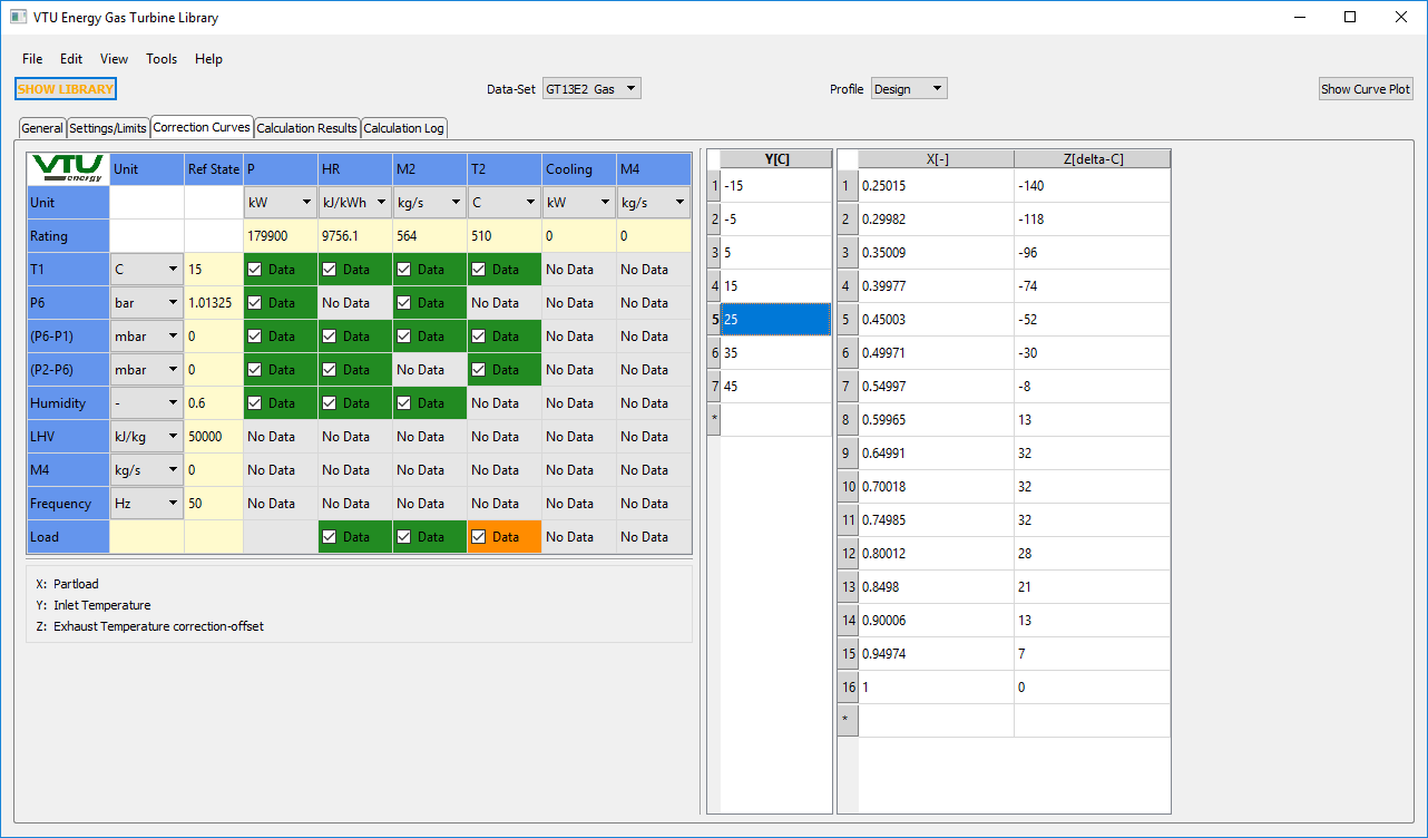
To select a specific curve, you have to double-click in the respective field of the matrix. Upon selection, the data will be displayed in tabular format in the right-hand area of this window. For two-dimensional corrections the data in the format Z = f(X,Y) are structured such that a table Z = f(X) is assigned to each value of the parameter Y. In the plot display this structure is equivalent to an array of curves with the parameter Y.

Pressing the button "Show Curve Plot" that is located on the upper right side of the window, a curve plot of the selected correction curve is generated in a separate window with the values of the parameter Y displayed in the legend.

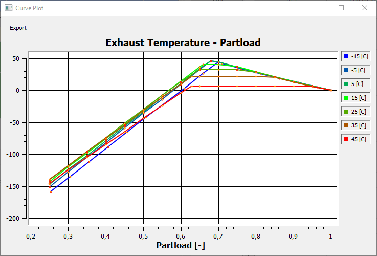
By clicking on the individual values of the legend, the respective X-Z curve can be hidden or re-activated in the plot, as for example the removal of all curves but the 25°C curve shown in the graph below.

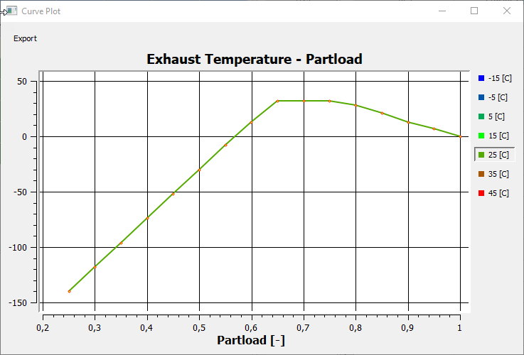
The plots remain linked to the data in the model and will update immediately, if data are changed in the underlying tables. Also, several plots can be opened at the same time, so that differences in e.g. the part load characteristics between different GT types can be analyzed graphically.

Data Input and Exchange to/from the Correction Curves

For adjusting the curve data, the user can directly edit or delete the cells of the tables, but one can also copy entire data sets between different curves (right-click menu in the matrix). All copy functions are also applicable in conjunction with Microsoft Excel.

Physics used

Modes including Corrections (FLOAD = 0,1,2)
Internal Calculations:
	Power Q = QN * Π CFQi Heat Rate HR = HRN * Π CFHRi Exhaust Flow M2 = M2N * Π CFM2i Exhaust temperature T2 = T2N + Σ COT2i QIN = Q1 + Q3 + Q4 QOUT = (Q + QLOSSAU)/ETAG + Q2 + Q8 EBD = (QIN - QOUT)/QIN
Equations:
	M2 = M2
	M3 = Q/(3600/HR*NCV3)
	M4 = M4N * Π CFM4i
	M1 = M2 - M3 - M4
	M5 = 1 ; //so that H5 = Q
	M8 = 1 ; //so that H8 = QCOOL
	H2 = f(T2,P2)
	H5 = Q
	H8 = QCOOL

Results

Besides the results relevant for the heat balance calculation which are displayed in the tab 'Results' of Component 106, the Gas Turbine Library also provides the results for each correction in a results table.

The overall correction is composed of the base load corrections and two further correction steps, viz. the part-load correction and the additional 'Manual Correction' defined by the user via the inputs for various correction factors in the specification values of Component 106. Finally, the correction for the difference in fuel temperature between the calculation case and the reference conditions of the data set is applied on the heat rate.

Component Displays

Display Option 1

Display Option 2

Example

Click here >> Component 106 Demo << to load an example.