Charlines (Characteristic curves)

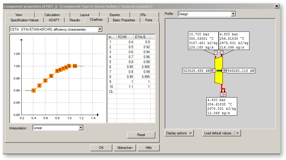
The combo box above the diagram shows a list of names of all characteristic curves of the selected component.

Select a characteristic curve with the left mouse button to see the points of the characteristic curve in the diagram and the table.

The number of points of a characteristic curve is variable.

Each characteristic curve can theoretically be defined completely differently in each profile. The inheritance of the values within the profiles is done as with the simple default values. Normally, however, a characteristic curve is defined in the design profile and transferred unchanged to all profiles.

On the X-axis of the diagram and in the middle column of the value table, the X-values of the characteristic curve are plotted or listed. These X-values must be specified in ascending order. The name of the X-values is in the table header above the middle table column and in the brackets () after =f of the characteristic curve name. In the example above FCHR.

The Y-values of the characteristic curve are plotted or listed on the Y-axis of the diagram and in the right column of the value table. The name of the Y-values is in the table header above the right-hand table column and on the left-hand side of the characteristic curve name, in each case before the fraction bar /. In the example above ETAI.

y = f (x) or ETAI = ETAIN * f (FCHR).

The names of the characteristic curves usually begin with a C, followed by the name of the y or result value of the characteristic curve.

Hint:

To ensure consistency between the design and partial load calculation, characteristic curves must run through the point (X=1,Y=1).

By default, linear interpolation is performed between the characteristic curve points. Outside the defined limits of the characteristic map, extrapolation is performed.

It is possible to set the interpolation mode to the following procedures (the effects are visible in the graphic in each case):

• linear interpolation
  In this mode, interpolation takes place within the characteristic curve range, outside the boundary value is retained (no extrapolation).
  
• Polynomial of any order
  In this mode, the degree of the polynomial can be specified for the interpolation within the characteristic curve range and for the extrapolation.
  
• Spline
  In this mode, the interpolation and extrapolation are carried out with the help of spline functions. There are the following setting options for the margins:
  • Third derivative (f'') = 0
  • setting of the first derivative (f') at the left and right edges
  • preset of the second derivative (f'') at the left and right margin

The change of the interpolation mode, however, only refers to characteristic curves where the y-value is read as a function of the x-value. Characteristic curves that are read "backwards" (x=f(y)) are basically only interpolated linearly. This applies to components 78, 79 (cooling towers), 84 (coal dryer), 86 (catalytic converter) and 94 (fan with characteristic diagram).

To change characteristic curve points, a row in the table must first be selected. This is done by clicking with the left mouse button in a cell of the desired row. Then another click in the field of the x-value or the y-value takes you to the editing mode and you can enter a new value.

Alternatively, it is possible to transfer characteristic data to Excel via the clipboard or from Excel to EBSILON®Professional. To do this, select the rows of the table to be transferred (pressing the Shift key enables selection of several rows) and click on "Copy" with the right mouse button. The data can then be transferred to Excel by clicking on "Paste". When importing, mark the area in Excel and click "Copy" and then in EBSILON®Professional. Select "Paste".

With the "Reset" button, all points of the displayed characteristic curve are reset to the values stored in the standard database. This button is only available in the design profile. If you are in a submenu, there is a "Delete" button there instead. If you click on "Delete", all values are set to those of the parent profile.

Characteristic curves are displayed graphically and can also be edited within the graphic:

• You can either click on the point on the curve or on the value in the table, both will then be marked.
  
• The following operations are possible via the right mouse button (context menu):
  
  • Edit curve (return to editing mode)
  • Zoom (to do this, the area to be enlarged must then be dragged with the left mouse button)
  • Move (in this mode the curve can be moved with the left mouse button)
  • Crosshair
  • Reset
  • Print
    
• Zooming is also possible by drawing a frame with the right mouse button
  
• Shifting the displayed area is also possible by holding down the middle mouse button.

 Press the "Help" button if you want help on the displayed characteristic curves.

Note: In the component properties window, unused points in characteristic curves are more clearly visible.

---

Result Array

Result arrays are characteristic curves that contain the results of a calculation.

They are used, among other things, for the solar components manifold and collector to graphically illustrate the status (pressure, pressure loss, temperature, enthalpy, mass flow) at the individual branch points, but also for some transient components such as components 119 and 126.

 

---

Characteristic fields (characteristic diagrams)

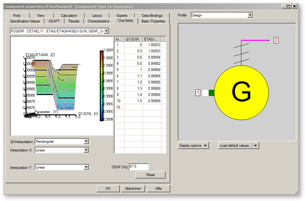
On this sheet, related characteristic curves of a component are displayed in a 3D chart.

Interrelated characteristic curves form a characteristic diagram.

Each characteristic curve of a field is assigned a parameter that is displayed below the value table and can be changed there.

The name of a field usually starts with FC, followed by the name of the parameter, e.g. FCH2P for component 11, which describes the efficiency ETAG (or z) as a function of the relative power Q1Q1N or Q2Q2N (or x) and as a function of the parameter H2P (hydrogen pressure in the generator housing) (or y).

z = f (x, y) or ETAG = ETAGN * f (Qx/QxN, H2P)

All characteristic curves of a characteristic diagram are also contained on the sheet Characteristic curves and can also be edited there.

The characteristic curves of a map must be specified in ascending order with regard to their parameter.

One of the characteristic curves of a map must go through the point through (X=1,Y=1), exactly the one that corresponds to the design value of the parameter. In the case of component 11, for example, this is the characteristic CETAEL2 for the standard set of values "standard" for the FCCOSPHI characteristic diagram. The nominal value of the parameter COSPHI is 0.85 here.

The characteristic fields sheet only appears for those components that have such interrelated characteristic curves.

This concerns at least the following components:

• component 11 generator
• component 57 gas turbine
• component 83 Pump (with characteristic diagram for speed)
• component 84 coal drying
• component 94 blower (with map)
• component 128 Hard coal mill
• component 129 Lignite mill

A characteristic field always has the same structure:
- the characteristic field X-values correspond to the X-values of the respective characteristic curve,
- the Y-values of the characteristic field correspond to the parameter values of the respective characteristic curve, and
- the characteristic field Z-values (result values of the characteristic diagram) correspond to the Y-values of the respective characteristic curve.

In this way, a three-dimensional XYZ-image can be formed, which represents the complete map in three dimensions.

If the component has result values after a successful simulation, the current result is also displayed as a point in this 3D chart.

When moving the mouse over the 3D chart, the tool tips for the objects located under the cursor (axes, lines, points, surfaces, etc.) are displayed. The following actions can be activated or carried out via the context menu of the 3D chart

• Select: clicking on this menu item switches between the modes: selection and view change.
  • With selection, the view of the display remains unchanged, only the objects in the chart can be selected by clicking the mouse.
  • When changing the view, the user can change the view of the display by moving the mouse. The pressed
    • left mouse button - causes the rotation of the display.
    • Middle mouse button - the displacement of the representation in the screen plane
    • Right mouse button or turning the mouse wheel with the Ctrl key pressed - the scaling (enlargement / reduction) of the representation

• Print: this allows the current representation to be printed out
• Save as Bitmap: to save the current representation as a raster graphic in an external file.
• Reset: by clicking on this menu item the original view (scaling, axis rotation) of the representation is restored.
• Show field: additional representation of the map, e.g. to illustrate the interpolated points
  • As a network: the map is additionally represented as a network.
  • As a coloured surface: the map is displayed as a surface whose colour changes depending on the map Z-value, as an alternative to the network display. The corresponding colour scale is also displayed in the 3D chart.

Sheet "Charcteristic field": Interpolation of the characteristic field in X and Y direction:

The type of interpolation between the grid points and the extrapolation at the edges of the map can be set individually in X- and Y-direction.

The interpolation / extrapolation in X-direction corresponds to the interpolation / extrapolation of the characteristic curves of the map.

The settings for the interpolation / extrapolation are analogous to the settings in the sheet "Characteristic curves".

If the setting for the interpolation / extrapolation in the X-direction is changed in the "Maps" sheet, this change is adopted for all characteristics of the relevant map.

Sheet "Charcteristic field": Alternative 2D interpolation of the charcteristic field:

The maps were interpolated at right angles. This means that the interpolation in Y-direction was always carried out between the grid points with identical X-values and thus exactly parallel to the Y-axis. This method provides good results if all characteristic curves of the field have identical length in X-direction.

However, if the length of the characteristic curves differs, the situation arises at the edges that, for example, one characteristic curve is still long enough and is interpolated, while the other characteristic curve is somewhat shorter and is therefore extrapolated. This leads to undesired effects during interpolation.

To counteract this effect, an alternative normalised 2D interpolation is implemented in addition to the rectangular interpolation. This type of interpolation takes into account the length of the characteristic curves and delivers more plausible results at the edges. The normalised 2D interpolation is recommended for the fields whose characteristic curves have different lengths (number of points).