

This topic contains several sections which will discuss some standard modeling tasks a typical power plant simulation user could encounter.
The following items are described here and recommended solutions are given.
Approach specification in HRSG icons
Evaporator Pinch Point Specification
HRSG Feed Water Preheater Recirculation
HRSG Desuperheater Spray Flow Control
Feed Water Heater (Conventional) Setup and Typical Specifications
Accessing Profile Variables for Turning Components off
Accessing Model Data for Display
Modeling Multiple Identical Trains
This section describes an example on how to set up an economizer by specifying an exit degrees of sub cooling.
Exit degrees of sub cooling here means the amount of degrees below saturation temperature at hot water exit pressure.
The best component to choose for an economizer under most circumstances is component 61. A measuring point, component (component 46) is required as well for this setup. See a screen shot of such a (partial) model below as an example:
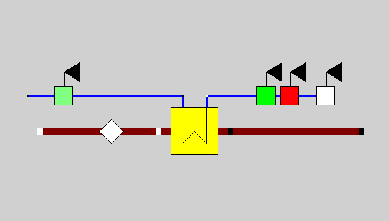
Component 33 is used in this case to specify flue gas inlet conditions and components type 46 to specify water inlet pressure, flow rate and temperature, the economizer requires an input that allow it to calculate both outlet conditions. One stream’s outlet enthalpy or temperature will be directly or indirectly specified and the other will follow from the mass and energy balance.
When looking through the inputs on the economizer, exit degrees of sub cooling is not an available option. However, there is a relatively simple way around this, using the method (4) shown in the screen shot below:
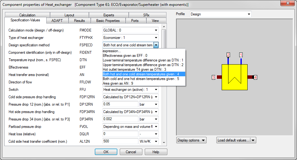
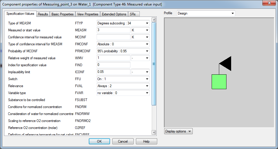
In case of method 4, steam inlet conditions and exit conditions must be specified, as well as one of inlet or outlet gas temperature. T2 would need to be specified (water exit temperature), but not in the field DTN. It must be specified externally. The exit water line has a component 46 placed on it. (measuring point). Instead of specifying the temperature there, the user can specify degrees of sub cooling. See the following screen shot.
This section describes an example on how to set up an economizer or super heater using the “approach” method.
The approach is defined as the difference between the incoming hot temperature (flue gas) and the outlet temperature of the heat exchanger’s cold flow (steam or water).
The methods used for this purpose are described below.
The best component to choose for an economizer or super heater under most circumstances is component 61. See a screen shot of such a (partial) model below as an example:
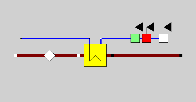
Using component 33 in this case to specify flue gas inlet conditions and components type 46 to specify water inlet pressure, flow rate and degrees sub cooling, the economizer requires an input that allow it to calculate both outlet conditions. One stream’s outlet enthalpy or temperature will be directly or indirectly specified and the other will follow from the mass and energy balance.
The approach can be specified as per the screen shot below:
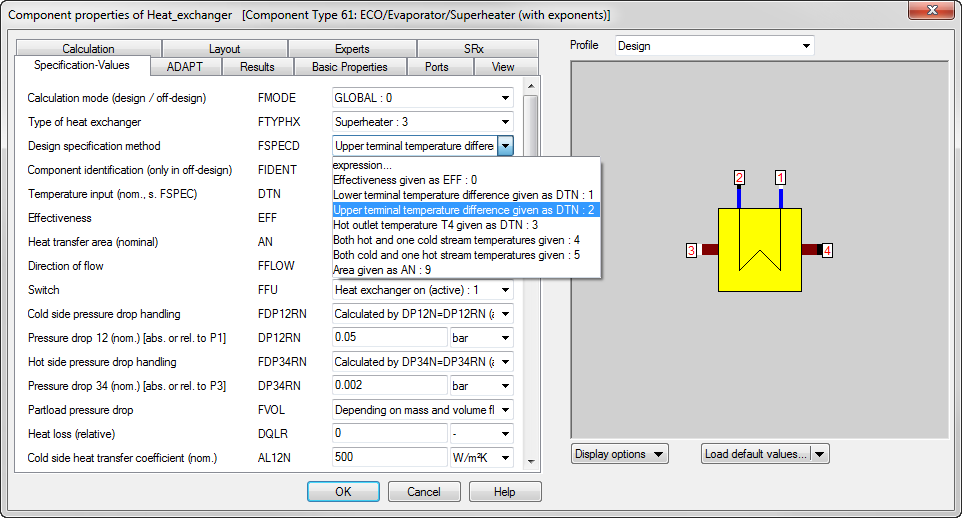
The type of heat exchanger is selected as 1 (economizer) or 3 (super heater). The selected Method is 2 (Upper terminal temperature difference given as DTN). This input for upper TTD represents the difference between the entering hot gas temperature and the leaving hot steam temperature.
The user specified approach will then be entered in the filed DTN.
This section describes an example on how to set up an evaporator using the pinch point approach.
It shows the components and methods used for this purpose.
The best component to choose for an evaporator under most circumstances is component 61, combined with a drum icon (component 20). See a screen shot of such a model below as an example:
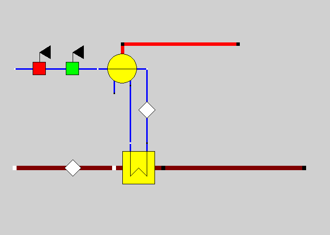
Using component 33 in this case to specify flue gas inlet conditions and components type 46 to specify water inlet pressure and temperature, the evaporator can determine the steam flow (in the red line) once the pinch point is specified.
Nevertheless the flow rate in the circulating loop between evaporator and drum must still be specified. This is the natural recirculation of the water-steam mixture. The steam will be wet vapour. The flow rate specified in the component 33 in this example defines the recirculating flow. The quality of the steam will be calculated based upon the user input for pinch point. The drum will then take the wet steam and separate out the steam to end up with the final steam production.
The pinch point is defined as per the screen shot below:

The method selected is 1. Lower TTD (terminal temperature difference) This represents the difference between the leaving cold gas temperature and the cold water temperature. However, since the water temperature is constant, this reflects the pinch point temperature.
The user specified pinch will then be entered in the field DTN.
This section describes an example on how to set up a desuperheater / temperature control mixer. It varies a water spray flow in order to regulate the downstream steam temperature.
A controller (component 39) is used to determine the water flow
Below is a screen shot of a (partial) model which uses a desuperheater.

Components of type 1 (boundary conditions) are used to determine the HRSG sections’ inlet conditions for both water and flue gas. The model furthermore contains an economizer (component 61), evaporator (component 61) with drum (component 20) and two super heaters (component 61). The economizer has its exit temperature determined by a measurement point (component 46), which is set to 10 degrees sub cooling at the pressure after the valve. The Evaporator’s circulating flow rate is set by a component 33. Both super heaters have their approach determined by settings inside the component itself.
Of most interest for this model however, are components 4, 38, and 39 (splitter, water injection mixer and controller). A Component 33 is used in the spray water flow line to 2 kg/s. This value will be the actual value if the controller is “off” and will be used as the start value for the controller if the controller is “on”.
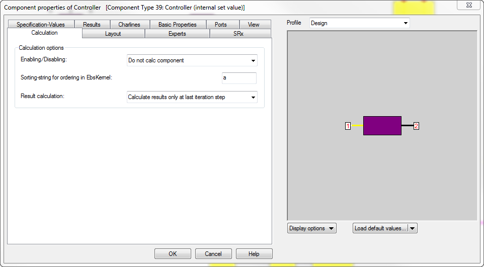
The off/on input for the controller can be found on the Calculation tab, see the screen shot below
As an alternative, variable FACT could have been used for the purpose of disabling the component by setting it to -1 or -2, see the screen shot below:
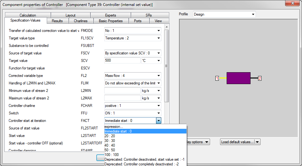
The benefit of using the variable FACT is that this variable can be set by way of expressions and can be used in scripts (see the topic on turning components off using preprocessor scripts further down)
Please ignore the value on line 2 (logic line) in this case, since the controller is disabled, this value is not updated.
The controller requires two connections, a black “logic” line and a yellow “actual” line. The logic line is connected to the variable to be modified in order to make the “actual” line value meet the internally specified target value.
The purpose of the controller is to limit the final super heater exit temperature to 500 °C. See the screen shot below:
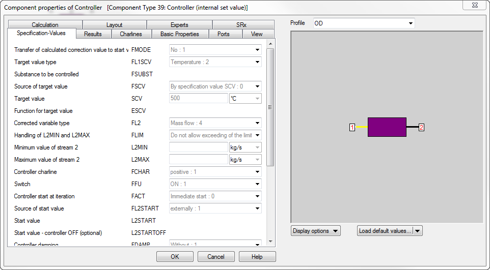
Notice that the start value for this controller is external as per setting for FL2START (this is the component 33, on the spray water line).
In a design case, the final super heater exit temperature is set by the design settings of the super heater itself. But in off-design, this will be calculated. If this number is not 500 °C, and the controller is on, then the spray flow will be adjusted by the controller. It will result in 0 kg/s, if the super heater exit temperature is less than 500C. But, in case it is higher than 500 °C, the spray flow will be adjusted by the controller, such that the final super heater becomes 500 °C.
This section describes an example on how to set up a HRSG recirculation control for the feed water preheater. It varies a recirculation flow in order to regulate the HRSG coldest inlet temperature. Such control are common to prevent the gas side condensation and corrosion at the coldest tubes.
A controller (component 39) is used to determine the recirculation water flow
Below is a screen shot of a (partial) model which uses a HRSG feed water recirculation controller.
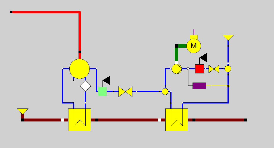
Components of type 1 (boundary conditions) are used to determine the HRSG sections’ inlet conditions for both water and flue gas. The model furthermore contains an economizer (component 61), evaporator (component 61) with drum (component 20). The economizer has its exit temperature determined by a measurement point (component 46), which is set to 10 degrees sub cooling at the pressure after the valve. The Evaporator’s circulating flow rate is set by a component 33. A pump with corresponding motor is used to circulate the warm water to preheat the HRSG inlet water. A Component 46, measurement point is used in the spray water flow line to set the pump exit pressure. The control valve of the pump will have its exit pressure automatically set equal to the HRSG inlet water pressure since they share a mixer, where the pressure must be equal.
Of most interest for this model however, are components 4, 37, and 39 (splitter, mixer and controller). This value will be the actual value if the controller is “off” and will be used as the start value for the controller if the controller is “on”.
The controller requires two connections, a black “logic” line and a yellow “actual” line. The logic line is connected to the variable to be modified in order to make the “actual” line value meet the internally specified target value.
The purpose of the controller is to increase the HRSG water inlet temperature to 90 °C. See the screen shot below:
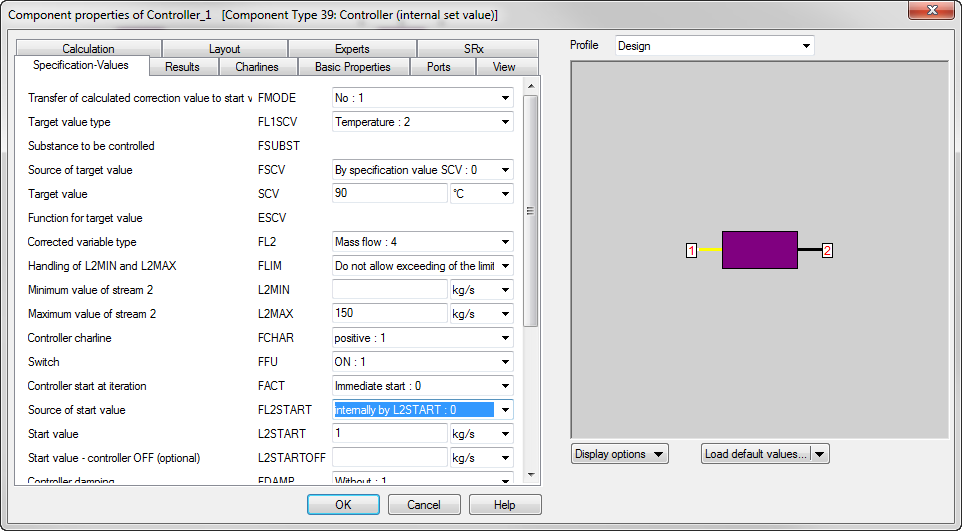
Notice that the start value for this controller is internal as per setting for FL2START and set to 1 kg/s
If HRSG water inlet temperature less 90 °C, and the controller is on, then the recirculation flow will be adjusted by the controller until the exit temperature of the mixer is 90 °C. The controller will result in 0 kg/s recirculation flow, if the HRSG water inlet temperature is higher than 90 °C.
This section describes an example on how to set up a typical feed water heater in a conventional plant.
A feed water heater in a conventional plant often contains a desuperheating section, a condensing section and a drain cooler section. The desuperheating section and drain cooler sections are sometimes not implemented.
In this example all three sections will be modelled. The recommended components and methods used for this purpose are described below.
In Ebsilon professional, it is required to use component 10 to model the condensing section of the feed water heater. Furthermore, this component can also model the desuperheating section. It is recommended that component 10 be used for the purpose of the modeling the desuperheater section as well, instead of the external desuperheater component (component 43). Component 10 does not model a drain cooler section though. If this is required, an additional component (27) called after cooler is best used. See the screen shot below for an example.
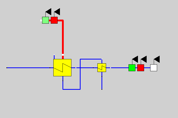
In this partial model the red line (steam) conditions are specified using degrees of superheat and pressure, as specified in two components 46. The cold feed water flow is specified along with pressure and temperature on the blue (water) line using three components 46. Drain cooler approach is specified in component 27 (on the right), and TTD is specified in component 10 (on the left). Component 10 models both the desuperheating section and the condensing section.
The reason that component 10 is best used for the purpose of modeling both the desuperheating section and condensing section, is that one needs to consider that in off-design conditions, the surface area used for desuperheating steam and the surface area for condensation change. The total area of course stays constant. But depending on load conditions, the desuperheating zone will transfer more or less heat and requires more or less surface area. The remainder of the surface area is then used for the condensing section. This change is significant, since the heat transfer coefficients for dry steam transferring heat to water and condensing steam transferring heat to water are different.
Component 10 estimates the impact of changes in heat transfer coefficients and changes in relative surface are per section, if the variable FRABEK is set =1 (yes). See the screen shot below for the sample model for this input variable.
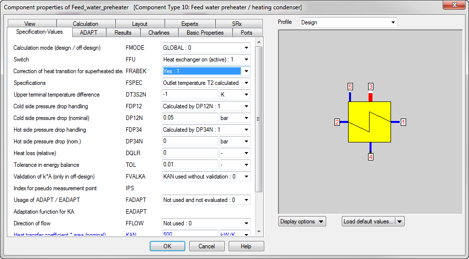
If there is no desuperheating section in the feed water heater, then FRABEK is best set to 0. In that case, of course a negative TTD is not correct. The (Upper) TTD in the example above = -1, which indicates that the water is heated to 1 degree above the saturation temperature of the extraction steam. Notice this is not the temperature difference between stream 3 and 2.
The drain cooler approach can be specified as per the screen shot below in component 27:
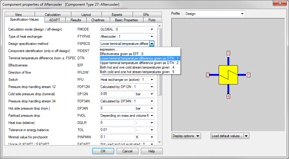
For FTYPHX the After Cooler: 1 is selected. AS Design specification method select 1: give lower terminal temperature difference. In case of a feed water heater, this is also more commonly known as the drain cooler approach. (= the difference in temperature between streams 4 (drain cooler outlet) and 1 (feed water inlet)).
The user specified approach will then be entered in the filed DTN (as default 5 degrees C).
This section describes an example on how to set up a gas turbine (component 106) running in part load.
Part loading of component 106 can be done by specifying the part load power or the part load fraction. Part load fraction is then defined as the fraction of the base load power given the current boundary conditions to the gas turbine. (so not as fraction or rated power).
A screen shot of a model using component 106 is below as an example:
Component 1 is used to define boundary conditions of the fuel, water/steam injection, and air conditions. In addition to this, measuring point (component 46) is used to specify the relative humidity. A piping loss (component 13) handles the inlet pressure drop. The GT back pressure is determined by another measuring point (component 46) in the flue gas line. Finally notice two logic lines, one for port 6, which tells the GT what the ambient pressure is which is required for correcting performance using correction curves. The second logic port is specifically used to allow for part loading the engine. A measuring point is located on this line, which sets the “enthalpy” of port 9. See the screen shot below for its settings:
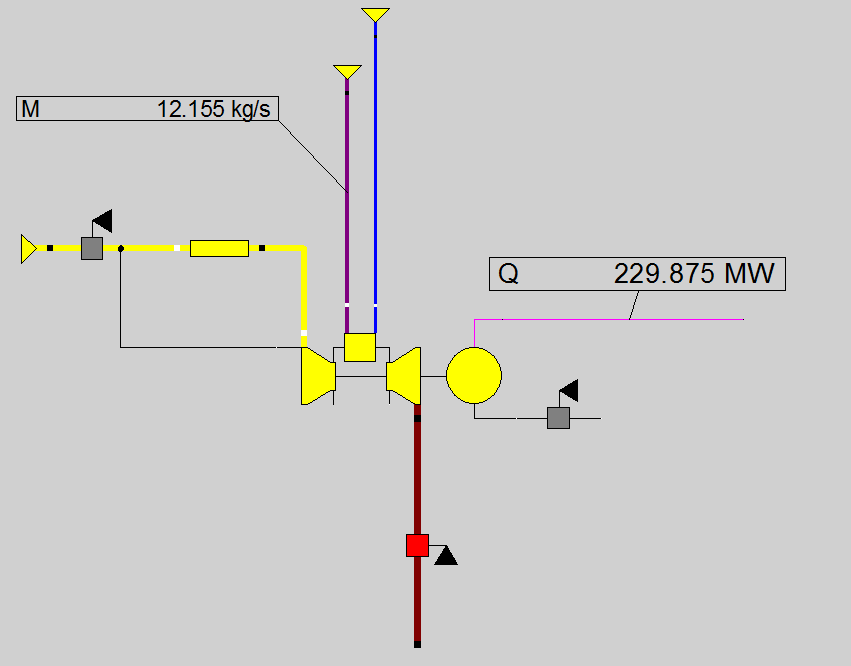
Part loading of component 106 by specifying the part load fraction can be done as follows:
Notice the input for MEASM on Logic port for load control Number 9 at the generator side = 0.8. This is a power/heat flow as per selection for FTYP. But it would have been possible to choose enthalpy as well:
There is no difference since the flow rate is by default 1. See the next screen shot for the pipe (logic line) values:
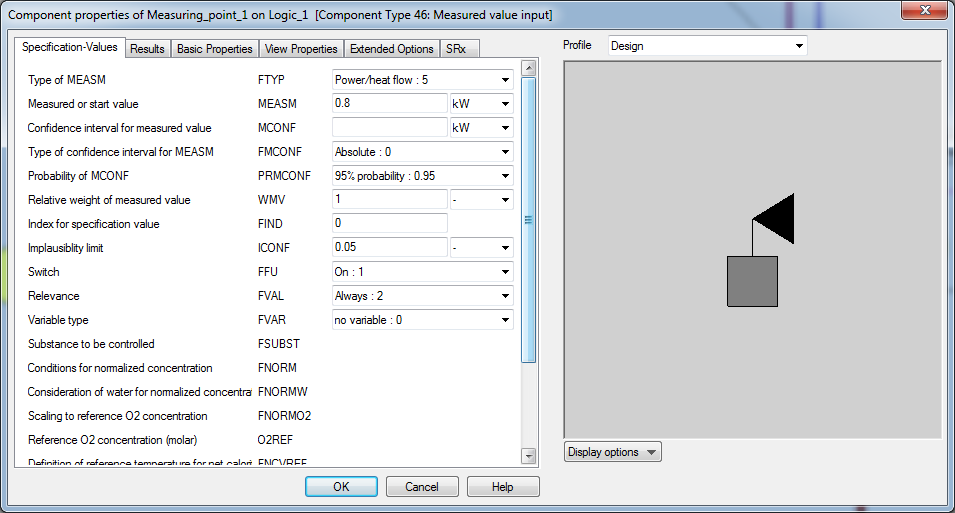
This input will only impact the gas turbine if the settings in the gas turbine are set up as follows:
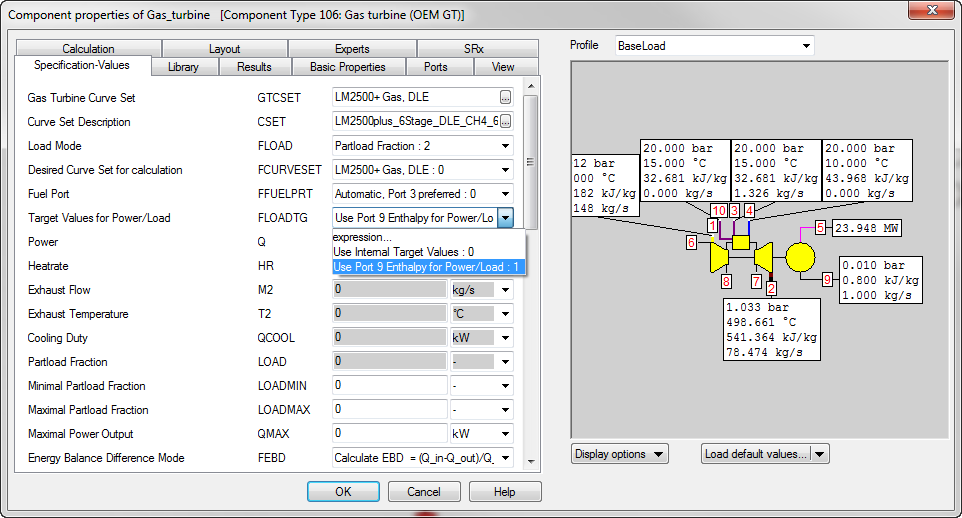
Notice the settings for FLOADTG =1 and FLOAD = 2 (part load fraction). In this setup, the load for the GT was 80% corresponding to the input of 0.8 on the measurement point on the logic line connected to port 9 of the GT. So, the 0.8 input here is not truly enthalpy or power, but will be interpreted as load fraction with the appropriate settings on the GT.
Notice the following setup for the Enthalpy is also possible for the measurement point:
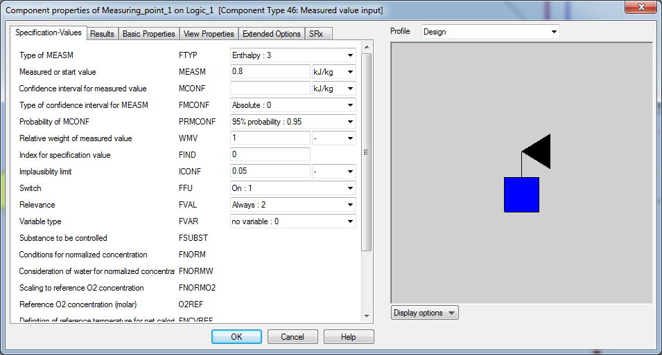
Part loading of component 106 by specifying the part load power can be done as follows:
The setup in the GT must then be as follows:
Notice FLOADTG is still 1 and FLOAD is set to 1, Desired Power.
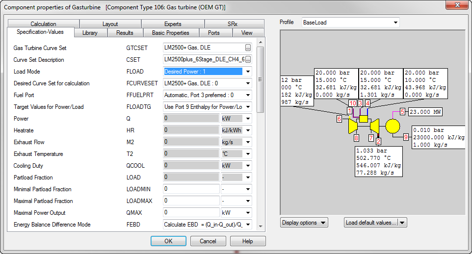
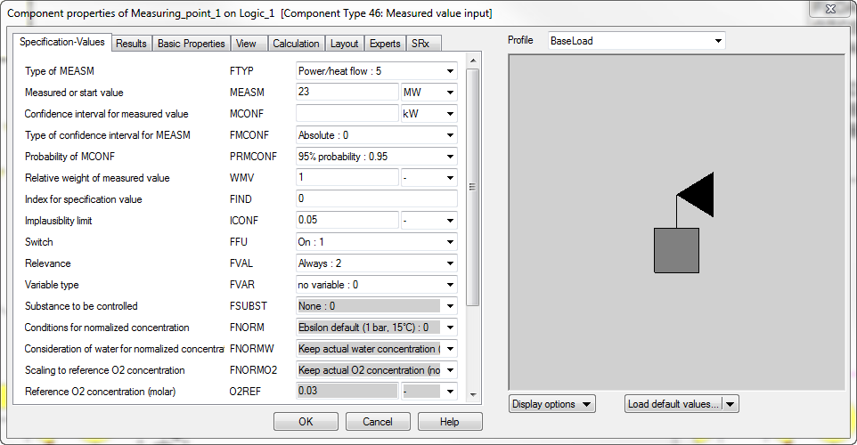
In this case the user can enter 23 MW in the measurement point on the logic line connected to port 9 of the GT.
This section describes an example on how to use user-defined profile variables to turn components on/off.
It shows how to use a profile variable to turn off components or controls, using the common FFU and FACT variables.
In this example a variable called HRSGOff is defined in the profile variables

The variable can be set to 0 to indicate the HRSG is off, or to 1 to indicate the variable is on.
The intention is the access this variable from the HRSG spray flow controller, and the super heater as well as evaporators and economizers.
The last three components have a variable FFU, which can take an expression as an input.
The expression has to evaluate to either 0 or 1 to be valid. The expression can be used as follows:
Use the @prof. portion of the expression to notify Ebsilon that a profile variable is accessed.
The @prof.HRSGOff variable is set to 0 (see the screen shot above).
FFU then becomes 0 as well and the component is bypassed, see the results in the screen shot below. Notice pressure drops are still considered.
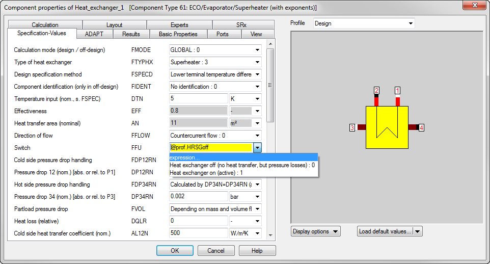
This expression can be used for all HRSG components that must be turned off. The benefit is that with only one input (a profile variable) the user can turn off all affected components.
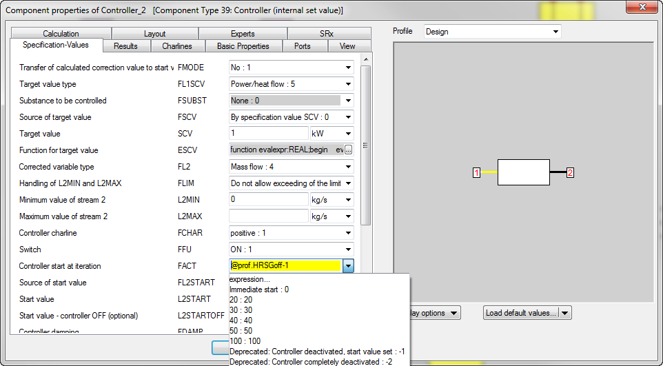
Similarly, the FACT variable can be used to turn controls off. In this case, the same variable can be used to turn it off. But FACT must evaluate to -1 or -2 to turn off the controller. See the screen shot below:
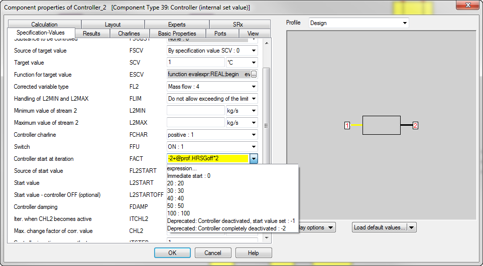
Some math will be required to turn an input of 0 for @prof.HRSGoff 0 into -2 and to turn an input of 1 for @prof.HRSGoff into 0 (see the screen shot above). Or to turn an input of 0 for @prof.HRSGoff 0 into -1 and to turn an input of 1 for @prof.HRSGoff into 0. See the screen shot below.
After running the model, the output can be seen:
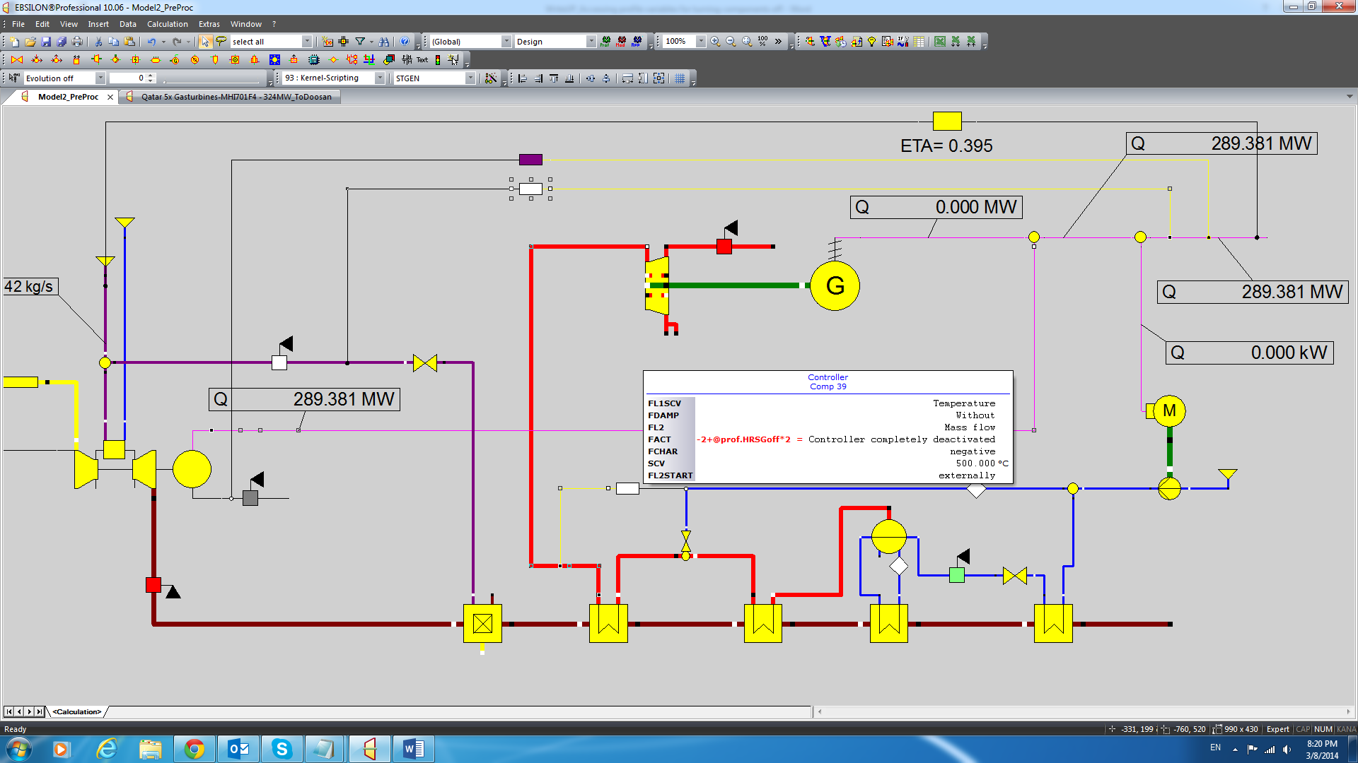
This section describes an example on displaying custom results.
It describes the use of text fields for the purpose of displaying customer’ defined results on the diagram or on a separate sheet. Furthermore, it shows the use of passive sheets and how to access variables from other components, stream variables and profile variables. One benefit of putting a table or text fields on a separate passive sheet is that the user can keep the zoom focused on the table. But the user may of course also put such text boxes on the Calculation sheet.
First, to add another sheet, you can right-click on the bottom ribbon. Select insert. See the screen shot below:
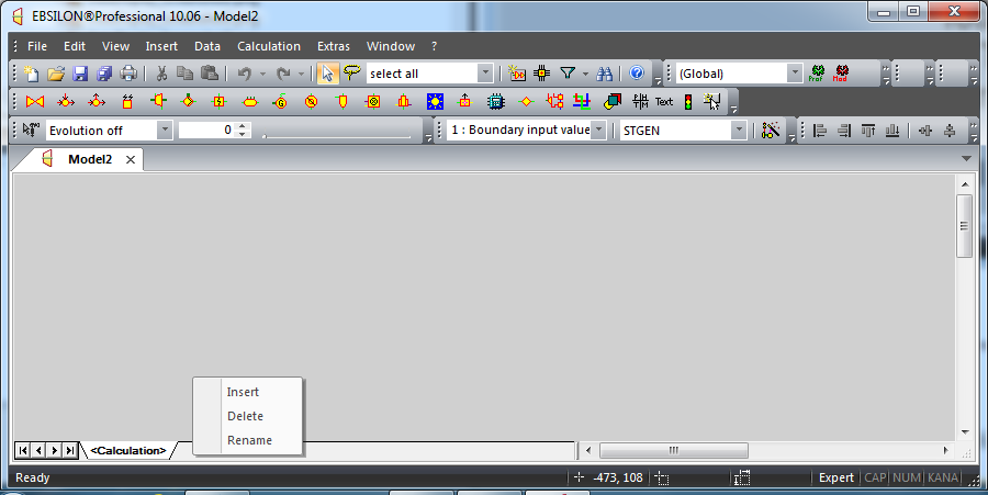
The default name will passive_sheet.
The sheet will not take part in any calculations, but does become part of the model.
The sheet can be used to display results for example.
To insert a text field (with one or multiple rows):
Insert Menu – Text Field
Once the text field is placed, you can enter simple text, such as in the screens shot below
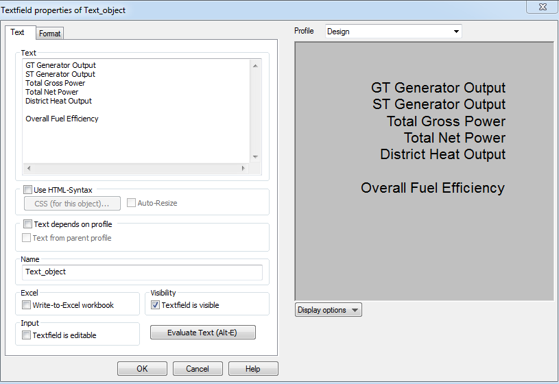
Or one can also insert user-defined expressions or formulae, such as those described in the following screen shot and the text below it:
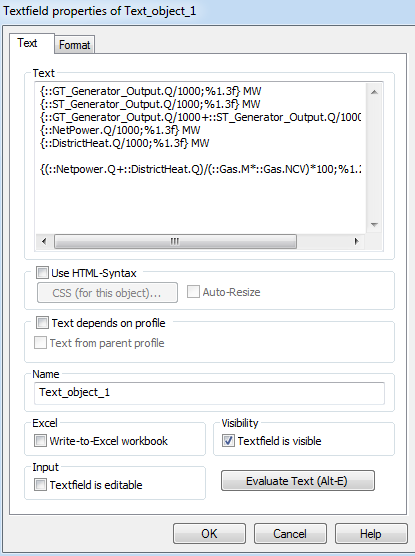
Or in more detail:
{::GT_Generator_Output.Q/1000;%1.3f} MW
{::ST_Generator_Output.Q/1000;%1.3f} MW
{::GT_Generator_Output.Q/1000+::ST_Generator_Output.Q/1000;%1.3f} MW
{::NetPower.Q/1000;%1.3f} MW
{::DistrictHeat.Q/1000;%1.3f} MW
{(::Netpower.Q+::DistrictHeat.Q)/(::Gas.M*::Gas.NCV)*100;%1.2f} %
The variables that are referenced here from the Gas stream (Gas.M and Gas.NCV) and from electric streams, such as: GT_Generator_Output, NetPower.Q, ST_Generator_Output.Q.
The format is defined as a floating point variable with 3 decimals display.
In this example, the formula (inside curly brackets) is followed by text such as MW or %.
Accessing streams or other variables can be done as on most input fields:
@prof.Var1 accesses user-defined profile variable called Var1
::Gas.T accesses the stream named “Gas”, variable named T (temperature).
::Generator1.QREAL accesses the component Generator1, variable QREAL.
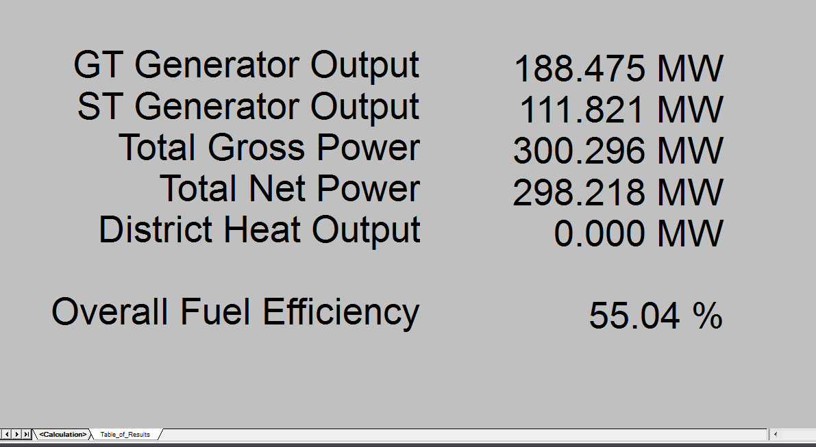
The final result will look something like this:
This section describes a few examples on how to set up a multiple identical trains (HRSG or ST for example). It uses flow multipliers and value transmitters. The example also shows how to calculate overall plant efficiency, how to sum up power and deduct auxiliary power requirements. Profile variables will be used as well.
Below is a screen shot of a (partial) model which models 3 Gas Turbines, 3 Heat Recover Steam Generators and 2 Steam Turbines. The HRSG and ST only model the HP section for simplicity.
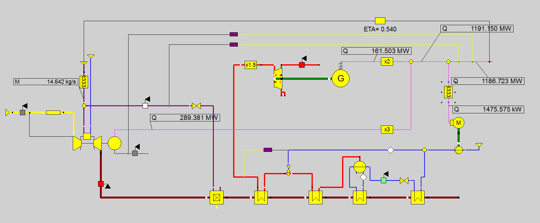
Components of type 1 (boundary conditions) are used to determine the HRSG water inlet conditions, ambient air conditions, fuel flow conditions and water/steam injection conditions. The model furthermore contains an economizer (component 61), evaporator (component 61) with drum (component 20) and two super heaters (component 61) with a desuperheater. The economizer has its exit temperature determined by a measurement point (component 46), which is set to 10 degrees sub cooling at the pressure after the valve. The Evaporator’s circulating flow rate is set by a component 33. The model also contains a duct burner. The measurement point on the logic line connected to port 9 sets the load of the GT. The controls for the desuperheater, net plant power as well as the use of port 9 for the GT are described in other examples.
In this example, we will focus on the use of flow multipliers and the use of a profile variables.
Two profile variables are defined: The first one represents the number of GTs and HRSGs, the second the number of STs. In this example 3 GTs and 2 STs are used. See the screen shot below:

These variables can be accessed from the flow multipliers. Notice there are flow multipliers in the fuel line, the GT power line, the ST power line, the HRSG steam line and the aux. power line. This allows the modeling of only 1 GT, 1HRSG and 1 ST and 1 Boiler Feed Pump, which will then provide the information needed to calculate the performance of the entire plant.
Profile variables can be used as pre-processor inputs. The equations or expressions on the input screens can then access these variables as follows: @prof.NumberOfSTs and @prof.NumberOfGTHRSGs.
An example for the GT power multiplier is shown below:
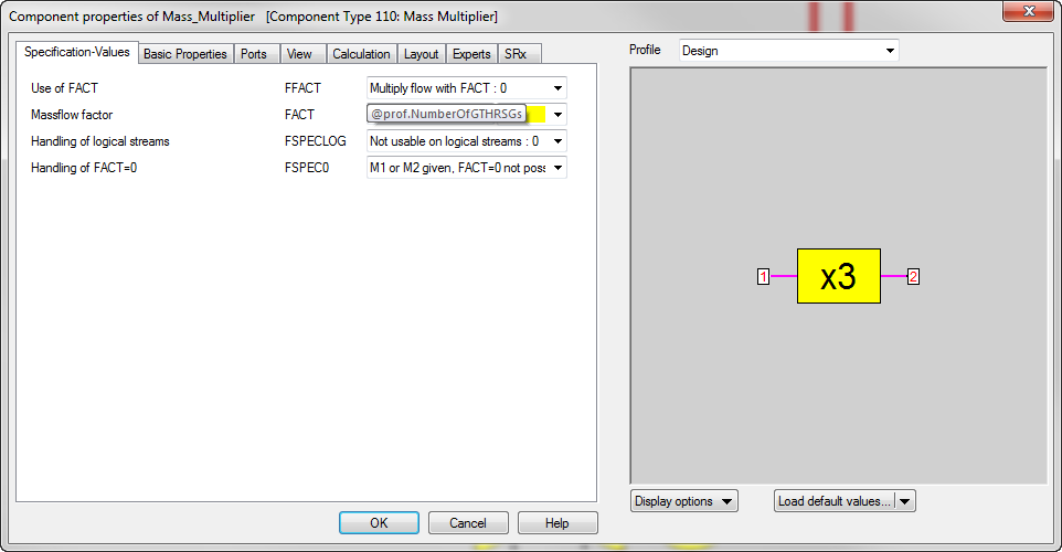
Another example to calculate the flow from the 3 HRSGs steam to the 2 STs is shown here. Notice two profile variables are accessed and basic math can be applied. In this case a division.
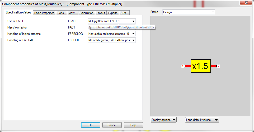
Similarly, the ST power multiplier (2), the boiler feed pump motor power multiplier (1/3) and the fuel multiplier (1/3) also use these profile variables.
Mixers are then used to mix the output of 3 GTs and 2 STs together and find the plant net power. (notice that for this example only the HP section of the steam turbine is modelled for simplicity sake, so power and efficiency may appear to be too low).
Finally, a component 32, efficiency meter is used to calculate plant efficiency. This component accesses the total fuel flow (duct burner and gas turbine combined for 3 units, 1/3rd of which is going to the GT which is actually modelled) and it accesses the combined ST and GT power, after reducing it by 3x the aux. power required for 1 boiler feed pump.
However, there is another way of modeling multiple trains which makes use of value transmitters. The same model above can also be modelled as follows, if a user wishes to model two STs separately, even though they are identical.
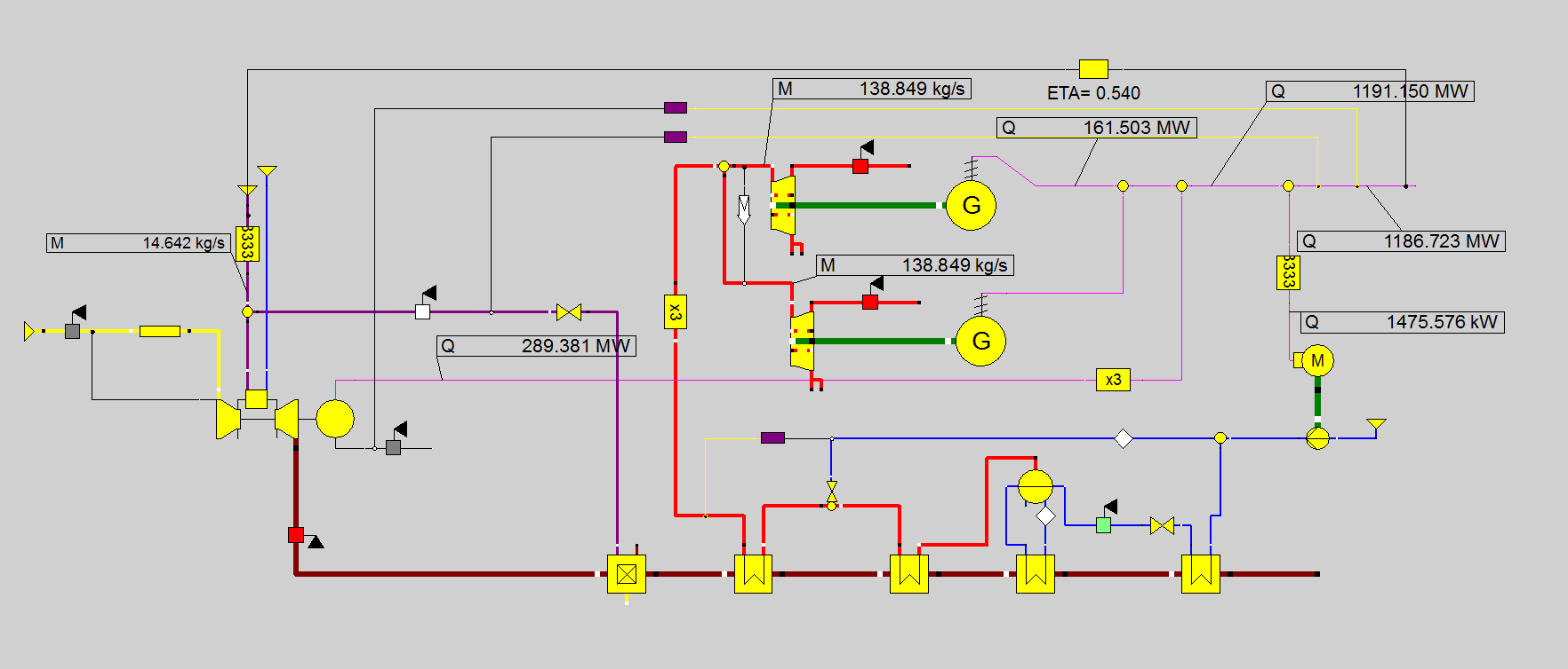
The results will be the same, but a value transmitter can be used to set the flow rate to one ST equal to the other. (or set it to 0 in case one ST is shut off.)
The setup of the value transmitter is as follows:
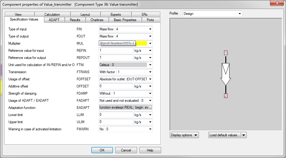
The multiplier in this case sets the 2nd ST flow equal to 0 (if only 1 ST is in operation) or equal to the 1st ST flow.
This section describes a few examples on how to set up power controls which vary duct firing or GT load fraction to meet a desired net plant power. The example also shows how to calculate overall plant efficiency, how to sum up power and deduct auxiliary power requirements.
Below is a screen shot of a (partial) model which models 3 Gas Turbines, 3 Heat Recover Steam Generators and 2 Steam Turbines. The HRSG and ST only model the HP section for simplicity.
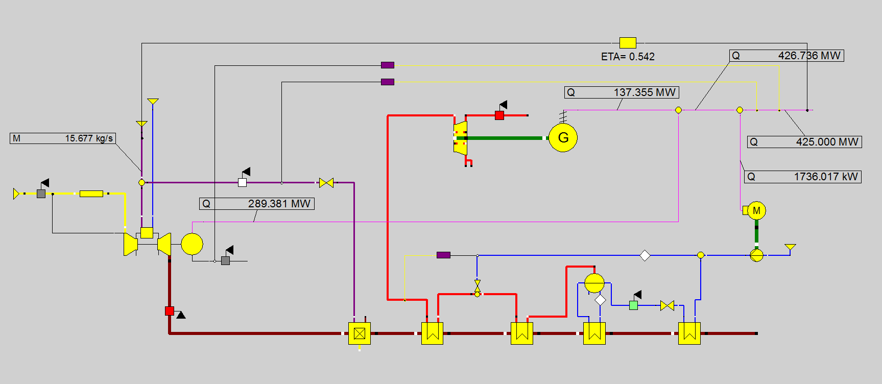
Components of type 1 (boundary conditions) are used to determine the HRSG water inlet conditions, ambient air conditions, fuel flow conditions and water/steam injection conditions. The model furthermore contains an economizer (component 61), evaporator (component 61) with drum (component 20) and two super heaters (component 61) with a desuperheater. The economizer has its exit temperature determined by a measurement point (component 46), which is set to 10 degrees sub cooling at the pressure after the valve. The Evaporator’s circulating flow rate is set by a component 33. The model also contains a duct burner. The measurement point on the logic line connected to port 9 sets the load of the GT. The controls for the desuperheater as well as the use of port 9 for the GT are described in other examples.
In this example, we will focus on the use of the two controls for net power.
Two different controls can be used: The first one varies the duct burner load to meet a net plant power demand, the second varies the GT load until the net plant power requirement is met.
Mixers are used to mix the power output of GT and ST together and find the plant net power, after sending some power to the motor which drives the boiler feed water pump.
Finally, a component 32, efficiency meter is used to calculate plant efficiency. This component accesses the total fuel flow (duct burner and gas turbine combined) and it accesses the calculated net plant power.
The setup of the duct burner control is as follows:

Notice the control is going to vary the flow connected to the logic line (black line) from port 2 (= duct burner flow) to match the actual line (yellow line) connected to port 1. That yellow line is connected to the portion of the pink line which represents net plant power. The target value = 425 MW, and the initial start value for the iteration is internally defined at 0 kg/s.
The setup of the GT load control is as follows:
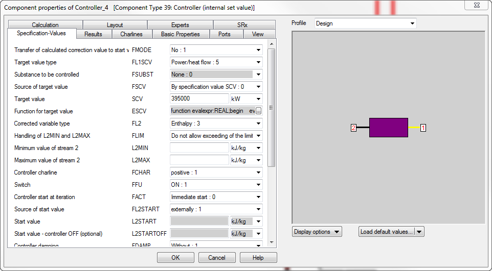
Notice the control is going to vary the “enthalpy” connected to the logic line (black line) from port 2 (= GT load) to match the actual line (yellow line) connected to port 1. That yellow line is connected to the portion of the pink line which represents net plant power. The target value = 395.5 MW, and the initial start value for the iteration is externally defined by the measuring point (component 46) located on the logic line connected to port 9 of the gas turbine. Recall that the gas turbine load can be externally controlled by using port 9’s enthalpy if the internal method to the GT is setup to take this value into account. See the screen shot below:
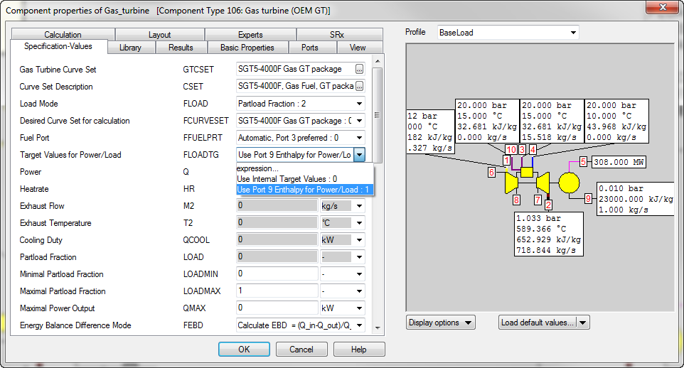
Of course in the example model at most one of the two controls can be activated at the same time, as they both attempt to control the same variable.