
EBSILON®Professional Online Documentation


|
Line connections |
|
|
General User Input Values Results Displays Example
This component allows to specify and calculate relevant wind data for one or several wind turbines (Component 143).
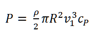
The relation between the power output P of a wind turbine, the undisturbed wind speed v1 at hub height, and the power coefficient cP is as follows:
For modern wind turbines, the hub height typically is at 100m or higher. As the undisturbed wind speed v1 as measured value at hub height is not available for a plant in the planning stage, it is calculated from existing data (mostly measurements at a height of 10m averaged over several years). Fig. 1 shows the schematic representation of the logarithmic vertical speed profile and the correlation between the wind speed values at different heights.
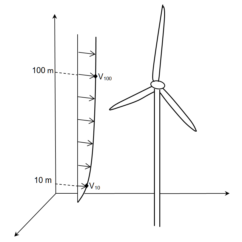
Fig. 1: Schematic representation of the logarithmic vertical speed profile assuming the Prandtl boundary layer
The calculation of the wind speed at hub height can be done according to various calculation algorithms. The most simple method is based on the assumption of a logarithmic vertical wind speed profile (Prandtl boundary layer, see Fig. 1). A complex algorithm additionally considers the influence of the atmospheric stability. This influence is related to the vertical temperature profile of the air near the ground. A distinction is made between three categories (see Fig. 2). In the case of the unstable stratification, the air close to the ground is warmer than the one above (typical of summer months with a strong heating of the ground). In the case of the stable stratification, the air temperature at the ground is lower than in the layers above (typical of winter months, when the ground cools off significantly). In the case of the neutral stratification, there is neither a warming nor a cooling in the air layer close to the ground. To consider the influence of the atmospheric stability, the data of the season, the position of the sun, and the cloud coverage data are required, among others. As these data are characteristic for a location, it is enough the carry out the calculations in one Component 142 and then adopt them for each wind turbine of a wind farm.
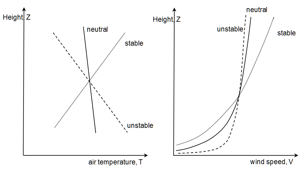
Fig. 2: The vertical temperature profile (left) and the corresponding wind speed profile (right) depending on the atmospheric stability
The calculation of the wind speed at hub height
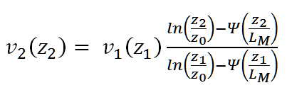
Algorithm 1: Calculation without considering the atmospheric stability (or for neutral stratification) assuming that the two heights z1 (the reference height at which the corresponding wind speed v1 is known) and z2 (the hub height) are located in the boundary layer (Fig. 1).
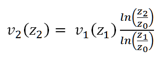
Here the roughness length z0, the heights z1 and z2, and the wind speed v1 are used as inputs. The result is the wind speed v2.
Algorithm 2: Improvement of Algorithm 1, consideration of the atmospheric stability.
Additional inputs are the total cloud overage in eights, months, and time of day, from which the position of the sun and the corresponding times for sunrise and sunset are determined. The previous formula is expanded by an empirical stability function Ψ as follows:
The stability function Ψ depends on the so-called Monin-Obukhov length LM and corrects the wind speed distribution by the corresponding temperature stratification. The precise form of the stability function Ψ can be found in [2]. The Monin-Obukhov length LM can be determined from the ground roughness length z0 and the dispersion category according to Klug/Manier, according to Table 17 from [3]. The dispersion category according to Klug/Manier in turn depends on the wind speed at a height of 10m, the total cloud coverage in eights, and the position of the sun (season, hours of night, hours of day, hours before and after sunrise/sunset). The algorithm described in [3] (Appendix A) is used for determining the dispersion category according to Klug/Manier.
[1] recommends the following values for the roughness length z0
| z0 [m] | Type of area |
| 2 | city centers |
| 1.5 | suburb areas |
| 0.3-1.6 | forest |
| 0.1 | heath land with trees and bush |
| 0.03 | farmland |
| 0.0001-0.001 | quiet water surface |
In Component 142, the Monin-Obukhov length LM can either be specified by the user directly or calculated on the basis of [3]-[4]. Subsequently, the Monin-Obukhov length from component 142 can be used in Components 143 for calculating the wind speed at hub height according to [2].
Table 17 from [3] for the determination of the Monin-Obukhov length LM depending on the dispersion category according to Klug/Manier and the roughness length z0 is shown below
| Dispersion category |
Roughness length z0 [m] |
||||||||
| acc. to Klug/Manier | 0.01 | 0.02 | 0.05 | 0.1 | 0.2 | 0.5 | 1.0 | 1.5 | 2.0 |
| I (very stable) | 7 | 9 | 13 | 17 | 24 | 40 | 65 | 90 | 118 |
| II (stable) | 25 | 31 | 44 | 60 | 83 | 139 | 223 | 310 | 406 |
| III/1 (neutral) | 99999 | 99999 | 99999 | 99999 | 99999 | 99999 | 99999 | 99999 | 99999 |
| III/2 (neutral) | -25 | -32 | -45 | -60 | -81 | -130 | -196 | -260 | -326 |
| IV (unstable) | -10 | -13 | -19 | -25 | -34 | -55 | -83 | -110 | -137 |
| V (very unstable) | -4 | -5 | -7 | -10 | -14 | -22 | -34 | -45 | -56 |
The geographic positions of the location are taken over from Component 117 (The sun). The same applies to the specification of the time when calculating with time series dialogs. From this the position of the sun and the dispersion category according to Klug/Manier are determined according to [4].
As in Component 143 (Wind turbine) the power characteristic of the manufacturer refers to the wind speed normalized according to IEC 61400-12-1, it is necessary to know the air temperature and air pressure required for the normalization according to IEC 61400-12-1. These values are also the same for all wind turbines of the wind farm and are therefore specified in one Component 142.
References
[1] Windkraftanlagen. Grundlagen, Entwurf, Planung und Betrieb. R. Gasch, J. Twele 8 Auflage (in German)
[2] VDI 3783 Blatt 8: Environmental meteorology – Turbulence parameters for dispersion models supported by measurement data (In German: Umweltmeteorologie Messwertgestützte Turbulenzparametrisierung für Ausbreitungsmodelle)
[3] Technische Anleitung zur Reinhaltung der Luft – TA Luft 2002 (In German)
[4] VDI 3782 Blatt 1: Environmental meteorology - Atmospheric dispersion models Gaussian plume model for air quality management (In German: Umweltmeteorologie Atmosphärische Ausbreitungsmodelle. Gauß’sches Fahnenmodell für Pläne zur Luftreinhaltung)
|
ISUN |
Index for solar data parameters (comp. 117) |
|
IWDATA |
Index for wind data parameters (current comp. 142 for usage in comp. 143) |
|
VWIND |
Wind speed |
|
AWIND |
Wind direction (from south to north =0°, positive in east direction) |
|
HVWIND |
Height specification for VWIND |
|
CLCOVE |
Cloud coverage in eighth |
|
VWIND10M |
Wind speed at 10 m height |
|
FLMO |
Monin-Obukhov length handling =0: Compute acc. to TA Luft, VDI 3782 Bl. 1 und VDI 3783 Bl. 8. from geo position (ISUN), CLCOVE, VWIND10M, Z0 =1: directly specified by LMO |
|
LMO |
Monin-Obukhov length |
|
PREF |
Reference air pressure |
|
TREF |
Reference air temperature |
|
Z0 |
Roughness length |
|
RLMO |
Computed Monin-Obukhov length |
|
DISPCAT |
Dispersion category acc. to Klug-Manier (see table for Monin-Obukhov length above) |
 |
Display option 1 |
Click here >> Component 142 Demo << to load an example.