
EBSILON®Professional Online Documentation


This example is taken from Chapter 7 of the Guideline VDI 2048, Sheet 2.
The example deals with the evaluation of the acceptance measurements before and after changing the LP-part turbines in a pressurized water nuclear power plant with the help of data validation according to the Guideline VDI 2048. The method is described there. The measurement values, estimated values for specifications and results are shipped on a CD.
Here, the handling of the example will be described by using Ebsilon.
1. Water-Steam cycle before retrofitting in simulation
First, the model is created and a design calculation is done with the specified data. The result is shown in Figure 10.
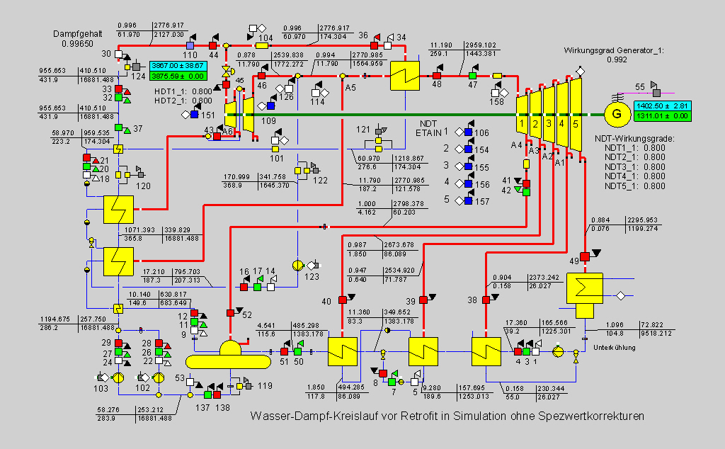
Figure 10
The high difference between the calculated generator power and its measured value is conspicuous. The reason can be found mainly in the too small turbine efficiency grades. Although the feed water measurement is also taken into account, but the specified confidence interval seems to be too big, because this measurement is calibrated with special care owing to the adherence to the approved maximum thermal reactor power. Because we have modelled this power plant in detail and supported it for many years (even during the retrofitting measures), exact knowledge of the plant is available, which would exceed the scope of the example calculation, but will be partly included in our check calculation.
As the most important change in the specification data, the isentropic efficiencies are adapted. For the high pressure turbine (2 discs) 0.90 and 0.88 are assumed, which match well with the manufacturer's measurements. For the low pressure discs, an isentropic efficiency of 0.88 is set. If the extraction temperature after the first disc is specified, then an isentropic efficiency of 0.755 results. For this reason, a pipe resistance of 1.2 bar before the turbine inlet and of 0.18 bar in the extraction is intended. The simulation calculation then also results in a value of 0.88 for the efficiency of the first low pressure disc. Figure 11 shows the simulation results.
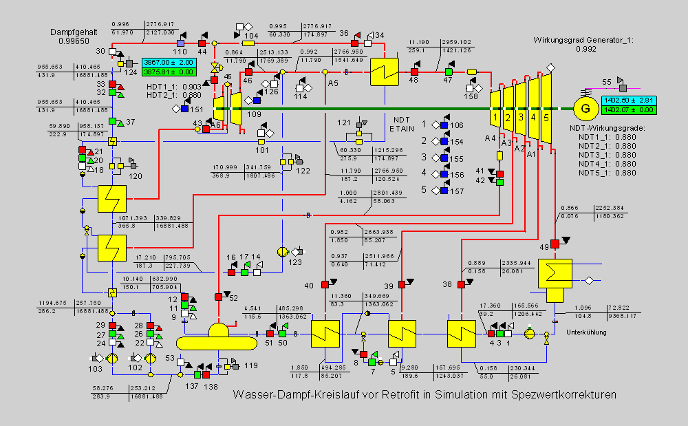
Figure 11
A good matching can be seen for the generator power. The following list of measurement values shows the measurement values and the related calculated values (SI-units).
Meas-point Meas.-value Calc. value Deviation [%]
-------------------------------------------------------
EtaiANZ1_1 0.88000 0.88000 0.00
EtaiANZ2_1 0.88000 0.88000 0.00
EtaiANZ3_1 0.88000 0.88000 0.00
EtaiAnz4_1 0.88000 0.88000 0.00
EtaiHDTA1_1 0.90300 0.90300 0.00
EtaiHDTA2_1 0.88000 0.88000 0.00
EtaiKond_1 0.88000 0.88000 0.00
mHDNK_1 660.470 705.904 -6.44 ?
mHK_1 1206.10 1206.44 -0.03
mKAVHDV_1 203.320 227.739 -10.72 ?
mKZUNKK_1 171.610 174.896 -1.88
mNKNDV_1 155.160 156.619 -0.93
mSPNP1_1 1077.86 1088.23 -0.95
mSPNP2_1 1038.79 1038.79 0.00
mSPVDE_1 2127.03 2127.03 0.00
mZUHD_1 178.880 174.896 2.28
mßISPWB_1 0.00000 0.00000 0.00
pADiK_1 0.07560 0.07560 0.00
pANZ1_1 0.15780 0.15780 0.00
pANZ2_1 0.63980 0.63980 0.00
pANZ3_1 1.85000 1.85000 0.00
pANZ4_1 4.16200 4.16200 0.00
pANZ6_1 23.3900 23.3900 0.00
pASPWB_1 4.01800 4.01800 0.00
Pel_1 1402500 1402066 0.03
pFDNFV_1 60.7300 60.7300 0.00
pFDVFV_1 61.9700 61.9700 0.00
pHDNK_1 10.1400 10.1400 0.00
pHDTA_1 11.7900 11.7900 0.00
pHK_1 17.3600 17.3600 0.00
pHKVSB_1 4.54100 4.54100 0.00
pKAVHDV_1 17.2100 17.2100 0.00
pKZUNKK_1 59.8900 59.8900 -0.00
pNKNDV_1 14.7500 14.7500 0.00
pNZU_1 11.1900 11.1900 0.00
PPuKLWA_1 190.000 175.809 8.07 ?
pSPNP1_1 81.9800 82.3700 -0.47
pSPNP2_1 82.3700 82.3700 0.00
PSpP1_1 10000.0 11508.6 -13.11 ?
PSpP2_1 10000.0 10985.6 -8.97 ?
pSPVDE_1 65.8900 65.8900 -0.00
psSPWB_1 3.81800 3.81800 0.00
PthDEn_1 3867000 3875813 -0.23
pZUHD_1 60.3300 60.3300 -0.00
qWVHDVW_1 60.0000 60.0000 -0.00
qWVKLWA_1 5.00000 5.00000 -0.00
qWVSPWB_1 20000.0 18214.5 9.80 ?
qWVZU_1 50.0000 50.0000 -0.00
tANZ4_1 172.500 172.500 0.00
tASPWB_1 139.941 139.941 -0.00
tHDNK_1 151.200 150.094 0.74
tHK_1 39.1600 39.1600 -0.00
tHKVSB_1 115.600 115.599 0.00
tKAVHDV_1 186.900 187.279 -0.20
tKZUNKK_1 222.600 222.933 -0.15
tNKNDV_1 88.3900 88.0153 0.43
tNZU_1 259.100 259.100 0.00
tSPNP1_1 143.600 141.218 1.69
tSPNP2_1 142.700 141.218 1.05
tSPNZUKK_1 222.550 222.159 0.18
tSPVDE_1 221.850 222.159 -0.14
xFDVFV_1 0.99650 0.99650 0.00
ßmEntn_1 0.94000 0.94000 0.00
ßpHWAZU_1 1.20000 1.20000 0.00
ßpKZUKK_1 0.44000 0.44000 0.00
ßpWAZU_1 0.60000 0.60000 0.00
ßpZUHDL_1 1.64000 1.64000 0.00
The strong deviations for the drying flow and the HP-auxiliary condensate are based on the measurement errors as per the experience. For the pump powers, only the estimated values are present, so that the calculated values are specified for the validation as estimated values. Otherwise, it can be seen that the simulation model maps the process very well. Thereby, Ebsilon makes sure that all balancing equations are maintained.
2. Water-steam cycle before retrofitting in validation
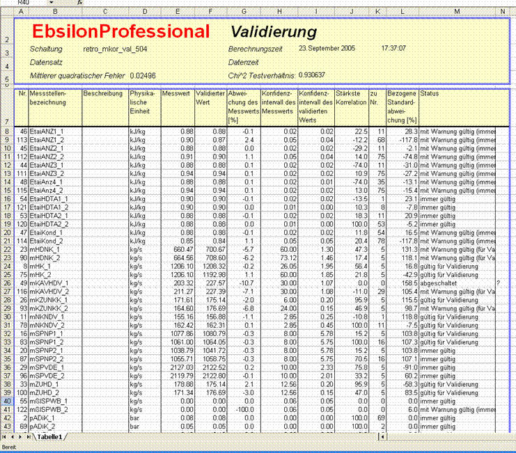
With the model obtained in the simulation including the specification values, the measurement values and a few specification data (drying ratio, turbine efficiency, pipeline resistance) are subject to data validation according to the Guideline VDI 2048 under consideration of the table uncertainties specified for the water/steam table IAPWS-IF97 (International Association for the Properties of Water and Steam, 2003). For the measurement values, for which the simulation shows a strong deviation, the confidence intervals were expanded accordingly. Else, the improvement of the CHI^2-test ratio, too big at the beginning, is achieved by measures described in the previous example of flow rate distribution (see also Guideline VDI 2048 Sheet 2). Figure 12 shows the results.
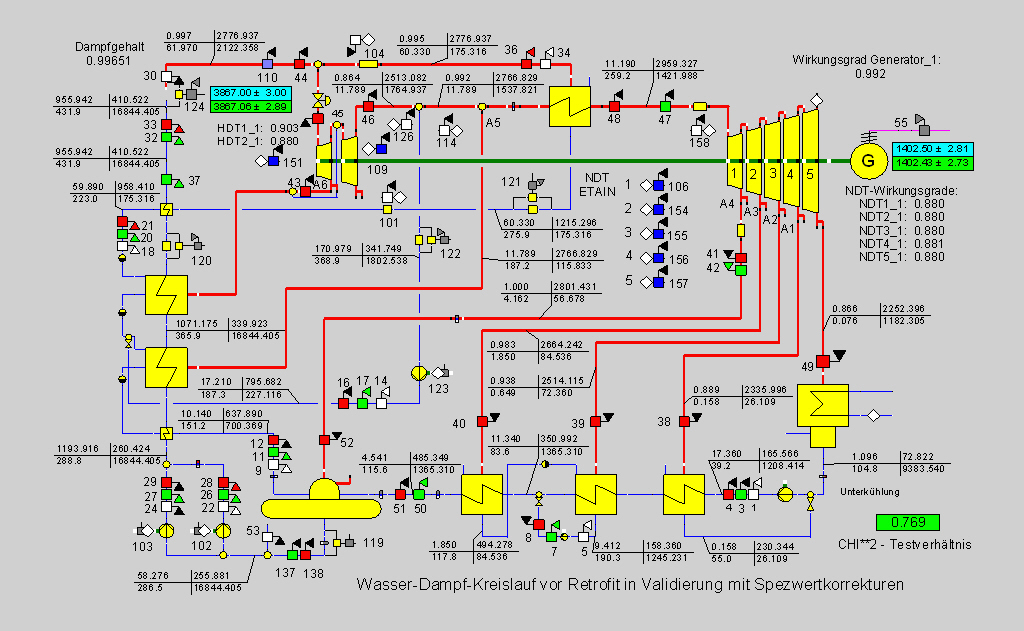
Figure 12
3. Water-Steam cycle after retrofitting in simulation
The method is the same as in the case of before retrofitting. The simulation carries out an adaptation of the isentropic efficiency for the low-pressure turbines. Thereafter, one gets the results displayed in Figure 13.
Figure 13
A glance at the list of the measurement values shows a big difference for the extraction temperature A4. The reason for this are the heat losses owing to missing insulation. After the insulation is integrated later, which was included by us in the model, the resulting temperature was about 20 K higher. For this reason, a correspondingly broad confidence interval must be set for validation.
4. Water-steam cycle after retrofitting in validation
After the adaptations resulting from the simulation calculations, first there is a CHI^2-test ration of above 40. The measures suggested in the guideline VDI 2048 for adjusting the confidence intervals finally lead to the result shown in Figure 14.
Figure 14
With that, good validation models are available for both the plant states.
5. Merging of the models
To be able to introduce correlations between the measurement values, which were made at the same place with the same instrumentation, both the calculation models for the states before and after retrofitting must be merged in a model i.e. both the plant states are merged in an Ebsilon model according to section 7.3 VDI 2048 Sheet 1 and are subject to a common validation. The correlation coefficients are taken from the VDI documentation of the example and are entered in the Ebsilon screen provided for this (Calculate\Covariance matrix). The next task is to calculate the probability for the fulfillment of the guarantee of an electrical power increase by 32 MW, further the power increase with a probability of 80%.
According to the description of the VDI example, the generator power is to be converted to a reference condenser pressure. Another correction results from the conversion to the reference steam generator power. The confidence intervals for the calculated quantities result from the error propagation law.
These additional calculations are handled in an EbsScript program.
// Program for Retrofit-Validation
// with conversion to nominal pressure and same DE-power
// and probability for maintaining the guarantee
var
ier: integer; // Error flag
i,j: integer; // Run-time variable
pgen1,pgen2: real; // Generator power
u1,u2: real; // Conversion factors for DE-power
delpgen: real; // Difference of generator powers
s1,s2,s: real; // Standard deviations
wn:array[1..11] of real; // Distribution function
zw:array[1..11] of real; // Abscissa values
arg: real; // Argument for distribution function
du,du1,du2,du3,du4: real; // Auxiliary quantities
wg: real; // Probability for guarantee fulfillment
pgen80: real; // Generator power with 80 % probability
qn: real; // Nominal DE-power
up1,up2: real; // Conversion factors to nominal pressure
dup1,dup2,sq: real; // Standard deviations
//
begin
// Distribution function of normal distribution
wn[1]:=0; // Integral values of normal distribution
wn[2]:=0.0013;
wn[3]:=0.0228;
wn[4]:=0.1587;
wn[5]:=0.3085;
wn[6]:=0.5;
wn[7]:=0.6915;
wn[8]:=0.8413;
wn[9]:=0.9772;
wn[10]:=0.9987;
wn[11]:=1;
zw[1]:=-1000; // Abscissa values
zw[2]:=-3;
zw[3]:=-2;
zw[4]:=-1;
zw[5]:=-0.5;
zw[6]:=0;
zw[7]:=0.5;
zw[8]:=1;
zw[9]:=2;
zw[10]:=3;
zw[11]:=1000;
//
qn:=3867000; // thermal nominal power
up1:= 1.0140; // Condenser pressure conversion factor for generator power
up2:= 0.9976;
// Confidence intervals for up1,up2
dup1:=0.0002;
dup2:=0.0002;
//
// Conversion of generator power
// to nominal waste steam pressure of 0.058 bar
pgen1:=Pel_1.result*up1;
pgen2:=Pel_2.result*up2;
// Confidence intervals of generator power
s1:=Pel_1.rconf;
s1:=s1*s1;
s1:=s1*up1*up1+Pel_1.result*Pel_1.result*dup1*dup1;
s2:=Pel_2.rconf;
s2:=s2*s2;
s2:=s2*up2*up2+Pel_2.result*Pel_2.result*dup2*dup2;
// Conversion to nominal DE-power of 3867 MW
u1:=qn/PthDEn_1.result;
u2:=qn/PthDEn_2.result;
pgen1:=pgen1*u1;
pgen2:=pgen2*u2;
// Difference of the converted generator powers
delpgen:=pgen2-pgen1;
// Error calculation
// Confidence intervals for the calculated generator power before retrofitting
sq:=PthDEn_1.rconf;
sq:=sq*sq;
du1:=qn/PthDEn_1.result;
du1:=du1*du1;
du2:=pgen1*qn/(PthDEn_1.result*PthDEn_1.result);
s1:=s1*du1+sq*du2;
// Confidence intervals for the calculated generator power after retrofitting
sq:=PthDEn_2.rconf;
sq:=sq*sq;
du1:=qn/PthDEn_2.result;
du1:=du1*du1;
du2:=pgen2*qn/(PthDEn_2.result*PthDEn_2.result);
s2:=s2*du1+sq*du2;
s:=sqrt(s1+s2);
// Probability for guarantee fulfillment
// Guarantee value = 32.1 MW
// Argument of the normal distribution function
arg:=(delpgen-32100)/s;
//print(arg);
j:=1;
i:=0;
wg:=0.9999;
while ((j > 0) and (i < 10)) do
begin
i:=i+1;
if arg < zw[i] then
begin
i:=i-1;
if i = 0 then
begin
wg:=0.0001;
end
else
begin
du:=(arg-zw[i])/2;
du1:=-zw[i]*zw[i]/2;
du1:=exp(du1);
du2:=-(zw[i]+du)*(zw[i]+du)/2;
du2:=exp(du2);
du3:=-(zw[i]+2*du)*(zw[i]+2*du)/2;
du3:=exp(du3);
du4:=sqrt(2*3.141593);
du4:=du/(3*du4);
du:=du4*(du1+4*du2+du3); // Simpson law
wg:=wn[i]+du;
if wg > 0.9999 then wg:=0.9999;
//print(" ",wg," ",wn[i]," ",du,"\n");
j:=0;
end;
end;
end;
// Performance enhancement with 80 % probability
// Argument of the distribution function for 80 % is 0.842
pgen80:=delpgen-s*0.842;
// Output
@model.error:=ier;
@prof.pgen1:=pgen1/1000;
@prof.pgen2:=pgen2/1000;
@prof.dpg:=delpgen/1000;
@prof.wgp:=wg*100;
@prof.ss:=s/1000;
@prof.pg80:=pgen80/1000;
@prof.profil:=getCalcProfileName;
end;
Figure 15 shows the final result.
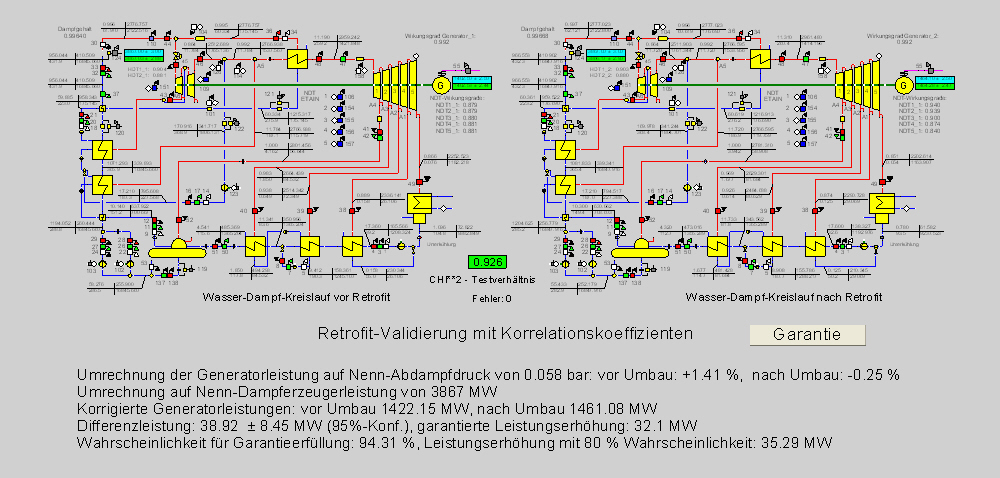
Figure 15
For analysis, a pre-defined Excel list can be created via Data àMeasurement Data àReport àValidation Results (Excel).
The measurement value ending "_1" identifies the measurement values before retrofitting , "_2" the values after retrofitting.
For each measurement value, a correlation list of the improvements can be printed (by a right-click with the mouse on the measurement value). For a specified minimum limit for the correlation coefficient of 0.1, one gets, for instance, the following list for the measurement point of main steam flow rate:
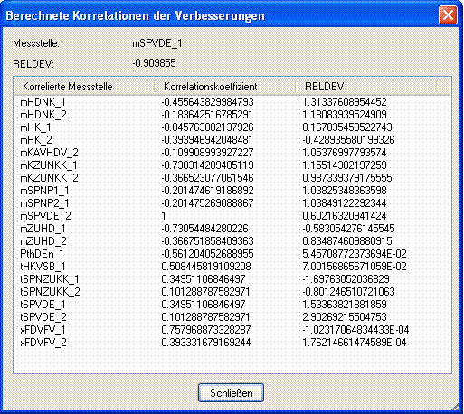
The list can be sorted on each heading of the columns.