
Flow rate distribution in a water-steam cycle
The example described in detail in the Appendix A of the Guideline VDI 2048 Sheet 1 is modelled and calculated with Ebsilon. To understand the individual calculation steps, it is recommended to read the cited Appendix A.
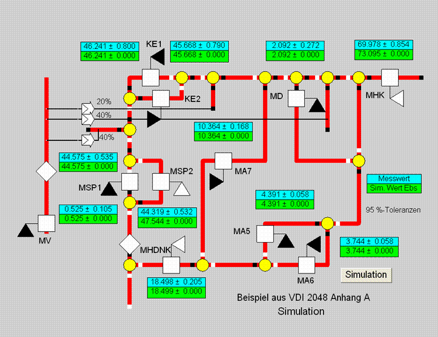
Because only mass flows are present, first a simple network model with splitting, mixing and pipelines is selected (see Figure 6).
Measurement values necessary for carrying out a simulation calculation, carry a filled component flag, whereas this is not the case with the redundant measurement values. The pseudo measurement points MFD and MZUE are not considered in the validation calculation, so that three redundant measurement values result. Another arrangement could also have been taken as the default value for the simulation (e.g. MHDNK instead of MA6).
The model, therefore, does not contain any components specific for the power plant. Steam is selected at all places as the pipeline type, which, however, is not relevant as far as the results are concerned.

Figure 6
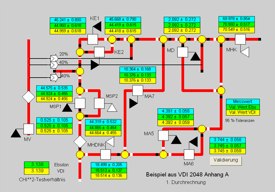
The simulation results of Figure 6 clearly show the deviations of the result values from the raw measurement values for the following redundant measurement values: Feed water flow rate MSP2 and back flow at the heating condenser MHK. These violations of the balance also become conspicuous in the validation. Figure 7 shows the results of the first run. A high matching can be seen in the validated values and the confidence intervals between the Ebsilon calculation and the VDI values.

Figure 7
The adaptation quality is expressed by the referred mean square error according to equation 140 of the Guideline VDI 2048 Sheet 1. This can be identified as Chi^2-Test. If one divides the variance by the 95%-quantile of the related F-distribution, then a value greater than 1 indicates high contradictions in the measured data. The value identified in Figure 7 as Chi^2-Test Ratio of 3.139 shows such a finding. Broad measurement errors are indicated in the comparative conditions equation 141 of the Guideline under consideration of the correlation of the improvements (correlation coefficients derived from the covariance matrix of the improvements).
The following table shows the referred deviations for measured values according to the equation 141 of the guideline VDI 2048 Sheet 1 and the respectively strongest correlation to another measurement value.
|
Measured value |
Criterion equation 141 |
Correlations coefficient |
Correlated measurement value |
|
Mfdke1 |
4.944 |
1.000 |
Mfdke2 |
|
Mfdke2 |
4.944 |
1.000 |
Mfdke1 |
|
Msp2 |
2.448 |
1.000 |
Msp1 |
|
Msp1 |
2.444 |
1.000 |
Msp2 |
|
Mhk |
1.649 |
0.140 |
Ma7 |
|
Ma7 |
0.223 |
1.000 |
Ma6 |
|
Mhdnk |
0.199 |
-0.967 |
Ma6 |
|
Ma5 |
0.149 |
1.000 |
Ma7 |
|
Ma6 |
0.149 |
-0.967 |
Mhdnk |
|
MV |
0.011 |
-0.873 |
Msp1 |
|
Md |
0.000 |
0.000 |
Md |
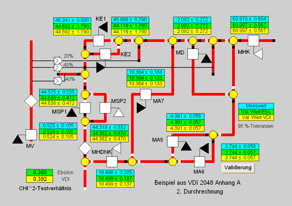
For the boiler and the feed water flow rates, the confidence intervals set in the empirical covariance matrix are too small. For the boiler flow rates, 2.5 kg/s is set instead of 0.8 kg/s for the second run according to the VDI template. Figure 8 shows a much improved Chi^2-test ratio of 0.392.

Figure 8
The control of the calculation runs and the evaluations is done by an EbsScript program in Pascal syntax. Since this programming language is integrated in Ebsilon, one or more such programs can be linked with each Ebsilon model (model and data) The VDI data were stored from the Appendix A of the Guideline in the EbsScript program and were thus displayed.
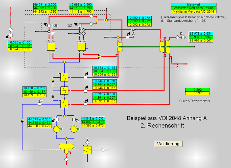
This example can also be calculated in a layout specific for the power plant.
The model of Figure 9 has pumps, heat-exchangers etc., the consequence of which is that sensible defaults must be made for calculating the pressure and the enthalpy.
This does not affect the mass flow, because no correlations regarding this are set. The results were expected to match.

Figure 9